Deep Learning 9_深度学习UFLDL教程：linear decoder_exercise（斯坦福大学深度学习教程）

前言

实验内容：Exercise:Learning color features with Sparse Autoencoders。即：利用线性解码器，从100000张8*8的RGB图像块中提取颜色特征，这些特征会被用于下一节的练习

理论知识：线性解码器和http://www.cnblogs.com/tornadomeet/archive/2013/04/08/3007435.html

实验基础说明：

1.为什么要用线性解码器，而不用前面用过的栈式自编码器等？即：线性解码器的作用？

这一点，Ng已经在讲解中说明了，因为线性解码器不用要求输入数据范围一定为(0,1），而前面用过的栈式自编码器等要求输入数据范围必须为(0,1）。因为a3的输出值是f函数的输出，而在普通的sparse autoencoder中f函数一般为sigmoid函数，所以其输出值的范围为(0,1)，所以可以知道a3的输出值范围也在0到1之间。另外我们知道，在稀疏模型中的输出层应该是尽量和输入层特征相同，也就是说a3=x1，这样就可以推导出x1也是在0和1之间，那就是要求我们对输入到网络中的数据要先变换到0和1之间，这一条件虽然在有些领域满足，比如前面实验中的MINIST数字识别。但是有些领域，比如说使用了PCA Whitening后的数据，其范围却不一定在0和1之间。因此Linear Decoder方法就出现了。Linear Decoder是指在隐含层采用的激发函数是sigmoid函数，而在输出层的激发函数采用的是线性函数，比如说最特别的线性函数——等值函数。

2.在实验中，在ZCA whitening前进行数据预处理时，每列代表一个样本，但为什么是对patches的每行0均值化（即：每一维度0均值化，具体做法是：首先计算每一个维度上数据的均值（使用全体数据计算），之后在每一个维度上都减去该均值。），而以前的实验都是对每列即每个样本0均值化（即：逐样本均值消减）？

①因为以前是灰度图，现在是RGB彩色图像，如果现在对每列平均就是对三个通道求平均，这肯定不行。因为不同色彩通道中的像素并不都存在平稳特性，而要进行逐样本均值消减（即：单独每个样本0均值化）有一个必须满足的前提：该数据是平稳的（见：数据预处理）。

平稳性的理解可见：http://lidequan12345.blog.163.com/blog/static/28985036201177892790。

②因为以前是自然图像，自然图像中像素之间的统计特性都一样，有一定的相关性，而现在是人工分割的图像块，没有这种特性。

3.在实验中，把网络权值显示出来为什么是用displayColorNetwork( (W*ZCAWhite)')，而不像以前用的是display_Network( (W1)')?

因为在本实验中，数据patches在输入网络前先经过了ZCA whitening的数据预处理，变成了ZCA白化后的数据ZCAWhite * patches，所以第一层隐含层输出的实际上是W*ZCAWhite * patches，也就是说从原始数据patches到第一层隐含层输出为W*ZCAWhite * patches的整个过程l转换权值为W*ZCAWhite。

4.PCA Whitening和ZCA Whitening的区别？即：为什么本实验没用PCA Whitening

PCA Whitening：处理后的各数据方差都都相等，并都为1。主要用于降维和去相关性。

ZCA Whitening：处理后的各数据方差不一定为1，但一定相等。主要用于去相关性，且能尽量保持原始数据。

5.优秀的编程技巧：

要学会用函数句柄，比如patches = bsxfun(@minus, patches, meanPatch);

因为不使用函数句柄的情况下，对函数多次调用，每次都要为该函数进行全面的路径搜索，直接影响计算速度，借助句柄可以完全避免这种时间损耗。也就是直接指定了函数的指针。函数句柄就像一个函数的名字，有点类似于C++程序中的引用。当然这一点已经在Deep Learning一之深度学习UFLDL教程：Sparse Autoencoder练习（斯坦福大学深度学习教程）中提到过，但我觉得有必须再强调一下。

实验步骤

1.初始化参数，编写计算线性解码器代价函数及其梯度的函数sparseAutoencoderLinearCost.m，主要是在sparseAutoencoderCost.m的基础上稍微修改，然后再检查其梯度实现是否正确。

2.加载数据并原始数据进行ZCA Whitening的预处理。

3.学习特征，即用LBFG算法训练整个线性解码器网络，得到整个网络权值optTheta。

4.可视化第一层学习到的特征。

实验结果

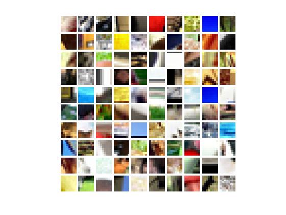
原始数据

ZCA Whitening后的数据

特征可视化结果，即：每一层学习到的特征

代码

linearDecoderExercise.m

%% CS294A/CS294W Linear Decoder Exercise
 
%  Instructions
%  ------------
%
%  This file contains code that helps you get started on the
%  linear decoder exericse. For this exercise, you will only need to modify
%  the code in sparseAutoencoderLinearCost.m. You will not need to modify
%  any code in this file.
 
%%======================================================================
%% STEP : Initialization
%  Here we initialize some parameters used for the exercise.
 
imageChannels = ;     % number of channels (rgb, so )
 
patchDim   = ;          % patch dimension
numPatches = ;   % number of patches
 
visibleSize = patchDim * patchDim * imageChannels;  % number of input units
outputSize  = visibleSize;   % number of output units
hiddenSize  = ;           % number of hidden units 
 
sparsityParam = 0.035; % desired average activation of the hidden units.
lambda = 3e-;         % weight decay parameter
beta = ;              % weight of sparsity penalty term       
 
epsilon = 0.1;           % epsilon for ZCA whitening
 
%%======================================================================
%% STEP : Create and modify sparseAutoencoderLinearCost.m to use a linear decoder,
%          and check gradients
%  You should copy sparseAutoencoderCost.m from your earlier exercise
%  and rename it to sparseAutoencoderLinearCost.m.
%  Then you need to rename the function from sparseAutoencoderCost to
%  sparseAutoencoderLinearCost, and modify it so that the sparse autoencoder
%  uses a linear decoder instead. Once that is done, you should check
% your gradients to verify that they are correct.
 
% NOTE: Modify sparseAutoencoderCost first!
 
% To speed up gradient checking, we will use a reduced network and some
% dummy patches
 
debugHiddenSize = ;
debugvisibleSize = ;
patches = rand([ ]);
theta = initializeParameters(debugHiddenSize, debugvisibleSize); 
 
[cost, grad] = sparseAutoencoderLinearCost(theta, debugvisibleSize, debugHiddenSize, ...
                                           lambda, sparsityParam, beta, ...
                                           patches);
 
% Check gradients
numGrad = computeNumericalGradient( @(x) sparseAutoencoderLinearCost(x, debugvisibleSize, debugHiddenSize, ...
                                                  lambda, sparsityParam, beta, ...
                                                  patches), theta);
 
% Use this to visually compare the gradients side by side
disp([numGrad grad]); 
 
diff = norm(numGrad-grad)/norm(numGrad+grad);
% Should be small. In our implementation, these values are usually less than 1e-.
disp(diff); 
 
assert(diff < 1e-, 'Difference too large. Check your gradient computation again');
 
% NOTE: Once your gradients check out, you should run step  again to
%       reinitialize the parameters
%}
 
%%======================================================================
%% STEP : 从pathes中学习特征 Learn features on small patches
%  In this step, you will use your sparse autoencoder (which now uses a
%  linear decoder) to learn features on small patches sampled from related
%  images.
 
%% STEP 2a: 加载数据 Load patches
%  In this step, we load 100k patches sampled from the STL10 dataset and
%  visualize them. Note that these patches have been scaled to [,]
 
load stlSampledPatches.mat  %怎么就就这个变量加到pathes上了呢？因为它里面自己定义了变量patches的值！
figure;
displayColorNetwork(patches(:, :)); 
 
%% STEP 2b: 预处理 Apply preprocessing
%  In this sub-step, we preprocess the sampled patches, in particular,
%  ZCA whitening them.
%
%  In a later exercise on convolution and pooling, you will need to replicate
%  exactly the preprocessing steps you apply to these patches before
%  using the autoencoder to learn features on them. Hence, we will save the
%  ZCA whitening and mean image matrices together with the learned features
%  later on.
 
% Subtract mean patch (hence zeroing the mean of the patches)
meanPatch = mean(patches, );  %为什么是对每行求平均，以前是对每列即每个样本求平均呀？因为以前是灰度图，现在是彩色图，如果现在对每列平均就是对三个通道求平均，这肯定不行
patches = bsxfun(@minus, patches, meanPatch);
 
% Apply ZCA whitening
sigma = patches * patches' / numPatches; %协方差矩阵
[u, s, v] = svd(sigma);
ZCAWhite = u * diag( ./ sqrt(diag(s) + epsilon)) * u';
patches = ZCAWhite * patches;
 
figure;
displayColorNetwork(patches(:, :));
 
%% STEP 2c: Learn features
%  You will now use your sparse autoencoder (with linear decoder) to learn
%  features on the preprocessed patches. This should take around  minutes.
 
theta = initializeParameters(hiddenSize, visibleSize);
 
% Use minFunc to minimize the function
addpath minFunc/
 
options = struct;
options.Method = 'lbfgs';
options.maxIter = ;
options.display = 'on';
 
[optTheta, cost] = minFunc( @(p) sparseAutoencoderLinearCost(p, ...
                                   visibleSize, hiddenSize, ...
                                   lambda, sparsityParam, ...
                                   beta, patches), ...
                              theta, options);
 
% Save the learned features and the preprocessing matrices for use in
% the later exercise on convolution and pooling
fprintf('Saving learned features and preprocessing matrices...\n');
save('STL10Features.mat', 'optTheta', 'ZCAWhite', 'meanPatch');
fprintf('Saved\n');
 
%% STEP 2d: Visualize learned features
 
W = reshape(optTheta(:visibleSize * hiddenSize), hiddenSize, visibleSize);
b = optTheta(*hiddenSize*visibleSize+:*hiddenSize*visibleSize+hiddenSize);
figure;
displayColorNetwork( (W*ZCAWhite)');

sparseAutoencoderLinearCost.m

function [cost,grad,features] = sparseAutoencoderLinearCost(theta, visibleSize, hiddenSize, ...
                                                            lambda, sparsityParam, beta, data)
%计算线性解码器代价函数及其梯度
% visibleSize:输入层神经单元节点数
% hiddenSize:隐藏层神经单元节点数
% lambda: 权重衰减系数
% sparsityParam: 稀疏性参数
% beta: 稀疏惩罚项的权重
% data: 训练集
% theta：参数向量，包含W1、W2、b1、b2
% -------------------- YOUR CODE HERE --------------------
% Instructions:
%   Copy sparseAutoencoderCost in sparseAutoencoderCost.m from your
%   earlier exercise onto this file, renaming the function to
%   sparseAutoencoderLinearCost, and changing the autoencoder to use a
%   linear decoder.
% -------------------- YOUR CODE HERE --------------------
% The input theta is a vector because minFunc only deal with vectors. In
% this step, we will convert theta to matrix format such that they follow
% the notation in the lecture notes.
W1 = reshape(theta(:hiddenSize*visibleSize), hiddenSize, visibleSize);
W2 = reshape(theta(hiddenSize*visibleSize+:*hiddenSize*visibleSize), visibleSize, hiddenSize);
b1 = theta(*hiddenSize*visibleSize+:*hiddenSize*visibleSize+hiddenSize);
b2 = theta(*hiddenSize*visibleSize+hiddenSize+:end);
 
% Loss and gradient variables (your code needs to compute these values)
m = size(data, ); % 样本数量
 
%% ---------- YOUR CODE HERE --------------------------------------
%  Instructions: Compute the loss for the Sparse Autoencoder and gradients
%                W1grad, W2grad, b1grad, b2grad
%
%  Hint: ) data(:,i) is the i-th example
%        ) your computation of loss and gradients should match the size
%        above for loss, W1grad, W2grad, b1grad, b2grad
 
% z2 = W1 * x + b1
% a2 = f(z2)
% z3 = W2 * a2 + b2
% h_Wb = a3 = f(z3)
 
z2 = W1 * data + repmat(b1, [, m]);
a2 = sigmoid(z2);
z3 = W2 * a2 + repmat(b2, [, m]);
a3 = z3;
 
rhohats = mean(a2,);
rho = sparsityParam;
KLsum = sum(rho * log(rho ./ rhohats) + (-rho) * log((-rho) ./ (-rhohats)));
 
squares = (a3 - data).^;
squared_err_J = (/) * (/m) * sum(squares(:));              %均方差项
weight_decay_J = (lambda/) * (sum(W1(:).^) + sum(W2(:).^));%权重衰减项
sparsity_J = beta * KLsum;                                    %惩罚项
 
cost = squared_err_J + weight_decay_J + sparsity_J;%损失函数值
 
% delta3 = -(data - a3) .* fprime(z3);
% but fprime(z3) = a3 * (-a3)
delta3 = -(data - a3);
beta_term = beta * (- rho ./ rhohats + (-rho) ./ (-rhohats));
delta2 = ((W2' * delta3) + repmat(beta_term, [1,m]) ) .* a2 .* (1-a2);
 
W2grad = (/m) * delta3 * a2' + lambda * W2;   % W2梯度
b2grad = (/m) * sum(delta3, );               % b2梯度
W1grad = (/m) * delta2 * data' + lambda * W1; % W1梯度
b1grad = (/m) * sum(delta2, );               % b1梯度
 
%-------------------------------------------------------------------
% Convert weights and bias gradients to a compressed form
% This step will concatenate and flatten all your gradients to a vector
% which can be used in the optimization method.
grad = [W1grad(:) ; W2grad(:) ; b1grad(:) ; b2grad(:)];
 
end
%-------------------------------------------------------------------
% We are giving you the sigmoid function, you may find this function
% useful in your computation of the loss and the gradients.
function sigm = sigmoid(x)
 
    sigm =  ./ ( + exp(-x));
end

displayColorNetwork.m

function displayColorNetwork(A)
 
% display receptive field(s) or basis vector(s) for image patches
%
% A         the basis, with patches as column vectors
 
% In case the midpoint is not set at , we shift it dynamically
if min(A(:)) >=
    A = A - mean(A(:)); % 0均值化
end
 
cols = round(sqrt(size(A, )));% 每行大图像中小图像块的个数
 
channel_size = size(A,) / ;
dim = sqrt(channel_size);   % 小图像块内每行或列像素点个数
dimp = dim+;
rows = ceil(size(A,)/cols);   % 每列大图像中小图像块的个数
B = A(:channel_size,:);                   % R通道像素值
C = A(channel_size+:channel_size*,:);    % G通道像素值
D = A(*channel_size+:channel_size*,:);  % B通道像素值
B=B./(ones(size(B,),)*max(abs(B)));% 归一化
C=C./(ones(size(C,),)*max(abs(C)));
D=D./(ones(size(D,),)*max(abs(D)));
% Initialization of the image
I = ones(dim*rows+rows-,dim*cols+cols-,);
 
%Transfer features to this image matrix
for i=:rows-
  for j=:cols-
 
    if i*cols+j+ > size(B, )
        break
    end
 
    % This sets the patch
    I(i*dimp+:i*dimp+dim,j*dimp+:j*dimp+dim,) = ...
         reshape(B(:,i*cols+j+),[dim dim]);
    I(i*dimp+:i*dimp+dim,j*dimp+:j*dimp+dim,) = ...
         reshape(C(:,i*cols+j+),[dim dim]);
    I(i*dimp+:i*dimp+dim,j*dimp+:j*dimp+dim,) = ...
         reshape(D(:,i*cols+j+),[dim dim]);
 
  end
end
 
I = I + ; % 使I的范围从[-,]变为[，]
I = I / ; % 使I的范围从[，]变为[, ]
imagesc(I);
axis equal  % 等比坐标轴：设置屏幕高宽比，使得每个坐标轴的具有均匀的刻度间隔
axis off    % 关闭所有的坐标轴标签、刻度、背景
 
end

参考资料

线性解码器

http://www.cnblogs.com/tornadomeet/archive/2013/04/08/3007435.html

http://www.cnblogs.com/tornadomeet/archive/2013/03/25/2980766.html