使用不同的机器学习方法进行预测

上篇2_Linear Regression and Support Vector Regression

高斯过程回归

%matplotlib inline 
import requests
from StringIO import StringIO
import numpy as np
import pandas as pd # pandas
import matplotlib.pyplot as plt # module for plotting
import datetime as dt # module for manipulating dates and times
import numpy.linalg as lin # module for performing linear algebra operations
from __future__ import division
import matplotlib
import sklearn.decomposition
import sklearn.metrics
from sklearn import gaussian_process
from sklearn import cross_validation
pd.options.display.mpl_style = 'default'

从数据预处理中读取数据

# Read in data from Preprocessing results
hourlyElectricityWithFeatures = pd.read_excel('Data/hourlyElectricityWithFeatures.xlsx')
hourlyChilledWaterWithFeatures = pd.read_excel('Data/hourlyChilledWaterWithFeatures.xlsx')
hourlySteamWithFeatures = pd.read_excel('Data/hourlySteamWithFeatures.xlsx')
dailyElectricityWithFeatures = pd.read_excel('Data/dailyElectricityWithFeatures.xlsx')
dailyChilledWaterWithFeatures = pd.read_excel('Data/dailyChilledWaterWithFeatures.xlsx')
dailySteamWithFeatures = pd.read_excel('Data/dailySteamWithFeatures.xlsx')
# An example of Dataframe
dailyChilledWaterWithFeatures.head()

	chilledWater-TonDays	startDay	endDay	RH-%	T-C	Tdew-C	pressure-mbar	solarRadiation-W/m2	windDirection	windSpeed-m/s	humidityRatio-kg/kg	heatingDegrees	occupancy
2012-01-01	0.961857	2012-01-01	2012-01-02	76.652174	7.173913	3.073913	1004.956522	95.260870	236.086957	4.118361	0.004796	7.826087	0.0
2012-01-02	0.981725	2012-01-02	2012-01-03	55.958333	5.833333	-2.937500	994.625000	87.333333	253.750000	5.914357	0.003415	9.166667	0.3
2012-01-03	1.003672	2012-01-03	2012-01-04	42.500000	-3.208333	-12.975000	1002.125000	95.708333	302.916667	6.250005	0.001327	18.208333	0.3
2012-01-04	1.483192	2012-01-04	2012-01-05	41.541667	-7.083333	-16.958333	1008.250000	98.750000	286.666667	5.127319	0.000890	22.083333	0.3
2012-01-05	3.465091	2012-01-05	2012-01-06	46.916667	-0.583333	-9.866667	1002.041667	90.750000	258.333333	5.162041	0.001746	15.583333	0.3

以上是我们的数据样本。

每日预测:

每日用电

获取训练/验证和测试集。dataframe显示功能和目标。

def addDailyTimeFeatures(df):
    df['weekday'] = df.index.weekday
    df['day'] = df.index.dayofyear
    df['week'] = df.index.weekofyear
    return df
dailyElectricityWithFeatures = addDailyTimeFeatures(dailyElectricityWithFeatures)
df = dailyElectricityWithFeatures[['weekday', 'day', 'week',
                                   'occupancy', 'electricity-kWh']]
#df.to_excel('Data/trainSet.xlsx')
trainSet = df['2012-01':'2013-06']
testSet_dailyElectricity = df['2013-07':'2014-10']
#normalizer = np.max(trainSet)
#trainSet = trainSet / normalizer
#testSet = testSet / normalizer
trainX_dailyElectricity = trainSet.values[:,0:-1]
trainY_dailyElectricity = trainSet.values[:,4]
testX_dailyElectricity = testSet_dailyElectricity.values[:,0:-1]
testY_dailyElectricity = testSet_dailyElectricity.values[:,4]
trainSet.head()

	weekday	day	week	occupancy	electricity-kWh
2012-01-01	6	1	52	0.0	2800.244977
2012-01-02	0	2	1	0.3	3168.974047
2012-01-03	1	3	1	0.3	5194.533376
2012-01-04	2	4	1	0.3	5354.861935
2012-01-05	3	5	1	0.3	5496.223993

以上是在预测每日用电时使用的特性。

交叉验证以获得输入参数 theta , nuggest

实际上有一些后台测试。首先做一个粗糙的网格serach参数，这里没有显示。之后，就可以得到精细网格搜索的参数范围，如下图所示。

def crossValidation_all(theta, nugget, nfold, trainX, trainY):
    thetaU = theta * 2
    thetaL = theta/2
    scores = np.zeros((len(nugget) * len(theta), nfold))
    labels = ["" for x in range(len(nugget) * len(theta))]
    k = 0
    for j in range(len(theta)):
        for i in range(len(nugget)):
            gp = gaussian_process.GaussianProcess(theta0 = theta[j], nugget = nugget[i])
            scores[k, :] = cross_validation.cross_val_score(gp,
                                                            trainX, trainY,
                                                            scoring='r2', cv = nfold)
            labels[k] = str(theta[j]) + '|' + str(nugget[i])
            k = k + 1
    plt.figure(figsize=(20,8))
    plt.boxplot(scores.T, sym='b+', labels = labels, whis = 0.5)
    plt.ylim([0,1])
    plt.title('R2 score as a function of nugget')
    plt.ylabel('R2 Score')
    plt.xlabel('Choice of theta | nugget')
    plt.show()
theta = np.arange(1, 8, 2)
nfold = 10
nugget = np.arange(0.01, 0.2, 0.03)
crossValidation_all(theta, nugget, nfold, trainX_dailyElectricity, trainY_dailyElectricity)

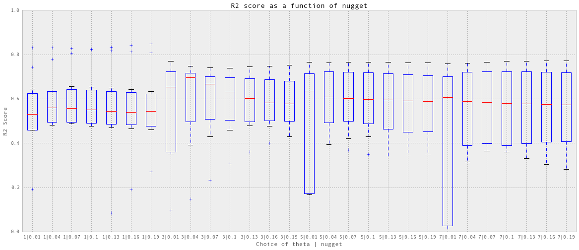
我选择theta = 3, nuggest = 0.04，这是最好的中位数预测精度。

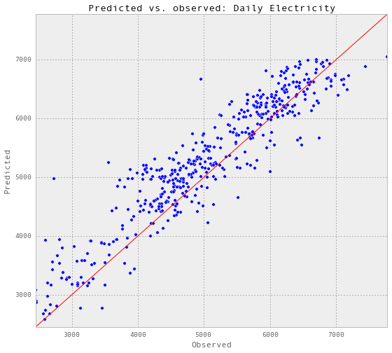
预测，计算精度和可视化

def predictAll(theta, nugget, trainX, trainY, testX, testY, testSet, title):
    gp = gaussian_process.GaussianProcess(theta0=theta, nugget =nugget)
    gp.fit(trainX, trainY)
    predictedY, MSE = gp.predict(testX, eval_MSE = True)
    sigma = np.sqrt(MSE)
    results = testSet.copy()
    results['predictedY'] = predictedY
    results['sigma'] = sigma
    print "Train score R2:", gp.score(trainX, trainY)
    print "Test score R2:", sklearn.metrics.r2_score(testY, predictedY)
    plt.figure(figsize = (9,8))
    plt.scatter(testY, predictedY)
    plt.plot([min(testY), max(testY)], [min(testY), max(testY)], 'r')
    plt.xlim([min(testY), max(testY)])
    plt.ylim([min(testY), max(testY)])
    plt.title('Predicted vs. observed: ' + title)
    plt.xlabel('Observed')
    plt.ylabel('Predicted')
    plt.show()
    return gp, results
gp_dailyElectricity, results_dailyElectricity = predictAll(3, 0.04,
                                                           trainX_dailyElectricity,
                                                           trainY_dailyElectricity,
                                 						   testX_dailyElectricity,
                                                           testY_dailyElectricity,
                                                           testSet_dailyElectricity,
                                                           'Daily Electricity')

Train score R2: 0.922109831389
Test score R2: 0.822408541698

def plotGP(testY, predictedY, sigma):
    fig = plt.figure(figsize = (20,6))
    plt.plot(testY, 'r.', markersize=10, label=u'Observations')
    plt.plot(predictedY, 'b-', label=u'Prediction')
    x = range(len(testY))
    plt.fill(np.concatenate([x, x[::-1]]),
             np.concatenate([predictedY - 1.9600 * sigma,
                             (predictedY + 1.9600 * sigma)[::-1]]),
             alpha=.5, fc='b', ec='None', label='95% confidence interval')
subset = results_dailyElectricity['2013-12':'2014-06']
testY = subset['electricity-kWh']
predictedY = subset['predictedY']
sigma = subset['sigma']
plotGP(testY, predictedY, sigma)
plt.ylabel('Electricity (kWh)', fontsize = 13)
plt.title('Gaussian Process Regression: Daily Electricity Prediction', fontsize = 17)
plt.legend(loc='upper right')
plt.xlim([0, len(testY)])
plt.ylim([1000,8000])
xTickLabels = pd.DataFrame(data = subset.index[np.arange(0,len(subset.index),10)], columns=['datetime'])
xTickLabels['date'] = xTickLabels['datetime'].apply(lambda x: x.strftime('%Y-%m-%d'))
ax = plt.gca()
ax.set_xticks(np.arange(0, len(subset), 10))
ax.set_xticklabels(labels = xTickLabels['date'], fontsize = 13, rotation = 90)
plt.show()

以上是部分预测的可视化。

每日用电预测相当成功。

每日冷水

获取训练/验证和测试集。dataframe显示功能和目标。

dailyChilledWaterWithFeatures = addDailyTimeFeatures(dailyChilledWaterWithFeatures)
df = dailyChilledWaterWithFeatures[['weekday', 'day', 'week', 'occupancy',
                                    'coolingDegrees', 'T-C', 'humidityRatio-kg/kg',
                                    'dehumidification', 'chilledWater-TonDays']]
#df.to_excel('Data/trainSet.xlsx')
trainSet = df['2012-01':'2013-06']
testSet_dailyChilledWater = df['2013-07':'2014-10']
trainX_dailyChilledWater = trainSet.values[:,0:-1]
trainY_dailyChilledWater = trainSet.values[:,8]
testX_dailyChilledWater = testSet_dailyChilledWater.values[:,0:-1]
testY_dailyChilledWater = testSet_dailyChilledWater.values[:,8]
trainSet.head()

	weekday	day	week	occupancy	T-C	humidityRatio-kg/kg	chilledWater-TonDays
2012-01-01	6	1	52	0.0	7.173913	0.004796	0.961857
2012-01-02	0	2	1	0.3	5.833333	0.003415	0.981725
2012-01-03	1	3	1	0.3	-3.208333	0.001327	1.003672
2012-01-04	2	4	1	0.3	-7.083333	0.000890	1.483192
2012-01-05	3	5	1	0.3	-0.583333	0.001746	3.465091

以上是用于日常冷水预测的特征。

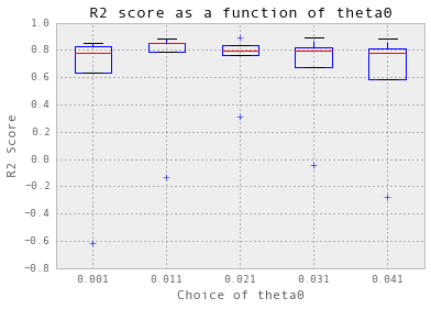
同样，需要对冷水进行交叉验证。

交叉验证以获得输入参数

def crossValidation(theta, nugget, nfold, trainX, trainY):
    scores = np.zeros((len(theta), nfold))
    for i in range(len(theta)):
        gp = gaussian_process.GaussianProcess(theta0 = theta[i], nugget = nugget)
        scores[i, :] = cross_validation.cross_val_score(gp, trainX, trainY, scoring='r2', cv = nfold)
    plt.boxplot(scores.T, sym='b+', labels = theta, whis = 0.5)
    #plt.ylim(ylim)
    plt.title('R2 score as a function of theta0')
    plt.ylabel('R2 Score')
    plt.xlabel('Choice of theta0')
    plt.show()

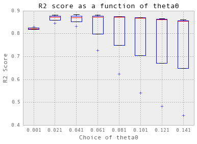
theta = np.arange(0.001, 0.1, 0.02)
nugget = 0.05
crossValidation(theta, nugget, 3, trainX_dailyChilledWater, trainY_dailyChilledWater)

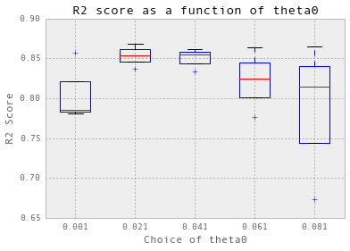
选择 theta = 0.021.

交叉验证实际上并不适用于冷冻水。首先，我必须使用三倍交叉验证，而不是十倍。此外，为了简化过程，从现在开始，我只显示针对theta的初始值的交叉验证结果:theta0。我在后台搜索了nugget。

预测，计算精度和可视化

theta = 0.021
nugget =0.05
# Predict
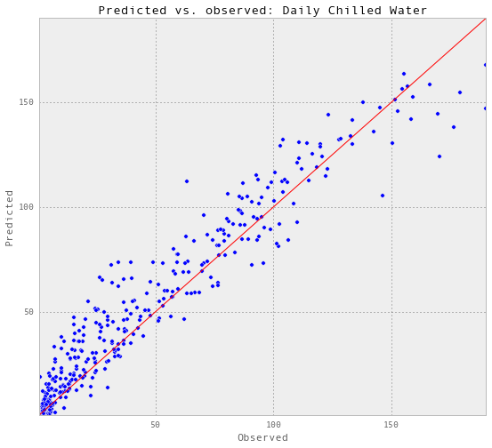
gp, results_dailyChilledWater = predictAll(theta, nugget,
                                           trainX_dailyChilledWater,
                                           trainY_dailyChilledWater,
                                           testX_dailyChilledWater,
                                           testY_dailyChilledWater,
                                           testSet_dailyChilledWater,
                                           'Daily Chilled Water')
# Visualize
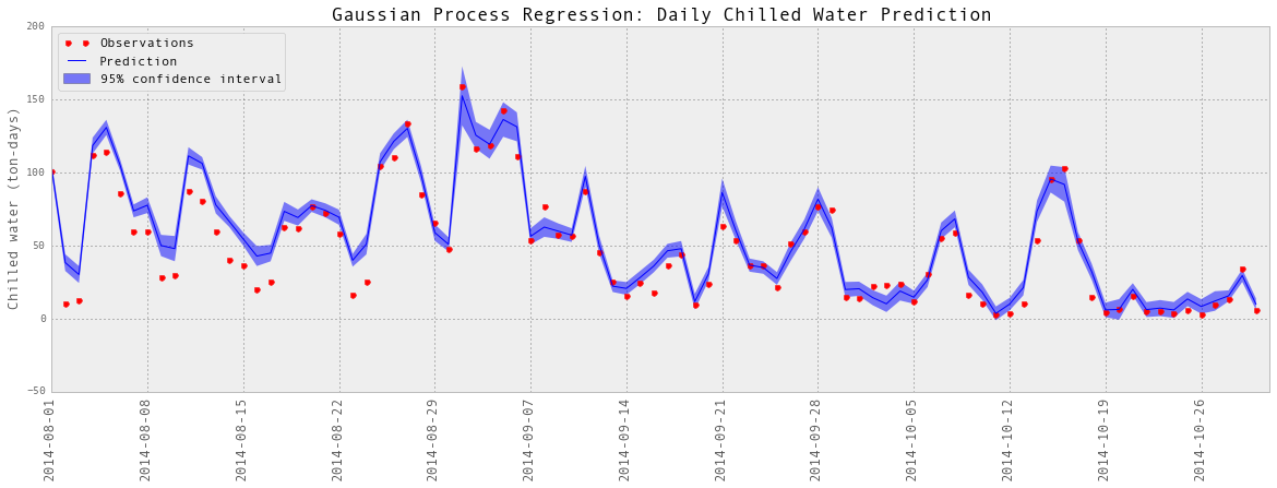
subset = results_dailyChilledWater['2014-08':'2014-10']
testY = subset['chilledWater-TonDays']
predictedY = subset['predictedY']
sigma = subset['sigma']
plotGP(testY, predictedY, sigma)
plt.ylabel('Chilled water (ton-days)', fontsize = 13)
plt.title('Gaussian Process Regression: Daily Chilled Water Prediction', fontsize = 17)
plt.legend(loc='upper left')
plt.xlim([0, len(testY)])
#plt.ylim([1000,8000])
xTickLabels = pd.DataFrame(data = subset.index[np.arange(0,len(subset.index),7)],
                           columns=['datetime'])
xTickLabels['date'] = xTickLabels['datetime'].apply(lambda x: x.strftime('%Y-%m-%d'))
ax = plt.gca()
ax.set_xticks(np.arange(0, len(subset), 7))
ax.set_xticklabels(labels = xTickLabels['date'], fontsize = 13, rotation = 90)
plt.show()

Train score R2: 0.91483040513
Test score R2: 0.901408621289

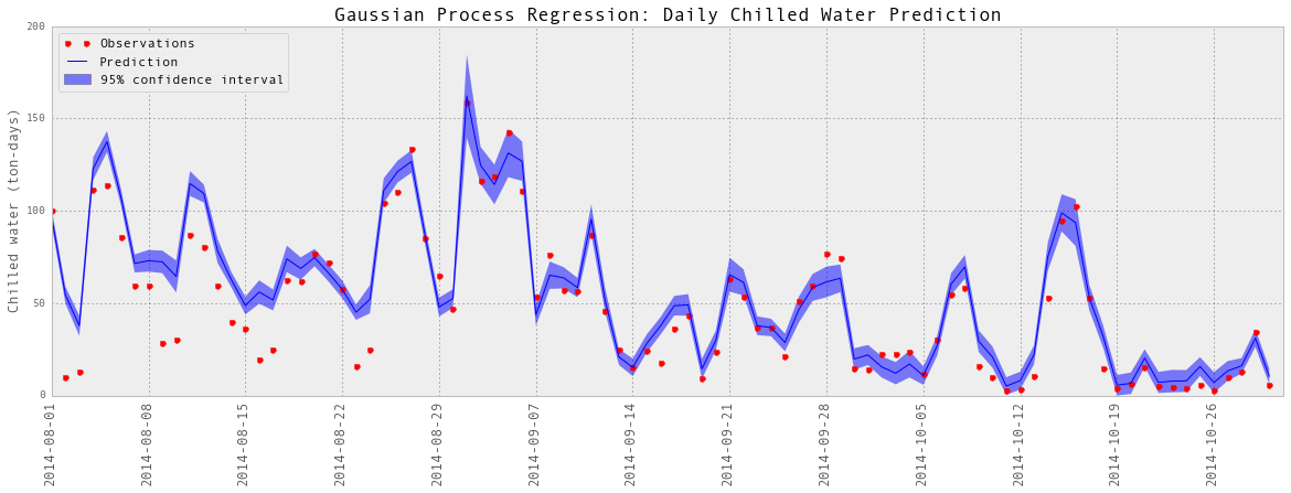
以上是部分预测的可视化。

预测又相当成功。

再增加一个特性:电量预测

为了提高预测精度，又增加了一个特性，即耗电量预测。预测的电量是根据前面电力部分中描述的时间特性产生的。这描述了入住计划。需要训练数据集中的实际用电量进行训练，然后将用电量作为测试数据集的特征进行预测。因此，这种预测方法仍然只需要时间和天气信息以及历史用电量来预测未来的用电量

dailyChilledWaterWithFeatures['predictedElectricity'] = gp_dailyElectricity.predict(
                                                            dailyChilledWaterWithFeatures[['weekday', 'day', 'week', 'occupancy']].values)
df = dailyChilledWaterWithFeatures[['weekday', 'day', 'week',
                                    'occupancy',
                                    'coolingDegrees', 'T-C',
                                    'humidityRatio-kg/kg',
                                    'dehumidification',
                                    'predictedElectricity',
                                    'chilledWater-TonDays']]
#df.to_excel('Data/trainSet.xlsx')
trainSet = df['2012-01':'2013-06']
testSet_dailyChilledWaterMoreFeatures = df['2013-07':'2014-10']
trainX_dailyChilledWaterMoreFeatures = trainSet.values[:,0:-1]
trainY_dailyChilledWaterMoreFeatures = trainSet.values[:,9]
testX_dailyChilledWaterMoreFeatures = testSet_dailyChilledWaterMoreFeatures.values[:,0:-1]
testY_dailyChilledWaterMoreFeatures = testSet_dailyChilledWaterMoreFeatures.values[:,9]
trainSet.head()

	weekday	day	week	occupancy	T-C	humidityRatio-kg/kg	predictedElectricity	chilledWater-TonDays
2012-01-01	6	1	52	0.0	7.173913	0.004796	2883.784617	0.961857
2012-01-02	0	2	1	0.3	5.833333	0.003415	4231.128909	0.981725
2012-01-03	1	3	1	0.3	-3.208333	0.001327	5013.703046	1.003672
2012-01-04	2	4	1	0.3	-7.083333	0.000890	4985.929899	1.483192
2012-01-05	3	5	1	0.3	-0.583333	0.001746	5106.976841	3.465091

交叉验证

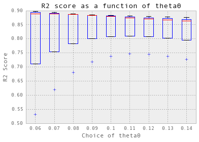
theta = np.arange(0.001, 0.15, 0.02)
nugget = 0.05
crossValidation(theta, nugget, 3, trainX_dailyChilledWaterMoreFeatures, trainY_dailyChilledWaterMoreFeatures)

选择 theta =0.021.

预测，计算精度和可视化

# Predict
gp, results_dailyChilledWaterMoreFeatures = predictAll(
    0.021, 0.05,
    trainX_dailyChilledWaterMoreFeatures,
    trainY_dailyChilledWaterMoreFeatures,
    testX_dailyChilledWaterMoreFeatures,
    testY_dailyChilledWaterMoreFeatures,
    testSet_dailyChilledWaterMoreFeatures,
    'Daily Chilled Water')
# Visualize
subset = results_dailyChilledWaterMoreFeatures['2014-08':'2014-10']
testY = subset['chilledWater-TonDays']
predictedY = subset['predictedY']
sigma = subset['sigma']
plotGP(testY, predictedY, sigma)
plt.ylabel('Chilled water (ton-days)', fontsize = 13)
plt.title('Gaussian Process Regression: Daily Chilled Water Prediction', fontsize = 17)
plt.legend(loc='upper left')
plt.xlim([0, len(testY)])
#plt.ylim([1000,8000])
xTickLabels = pd.DataFrame(data = subset.index[np.arange(0,len(subset.index),7)],
                           columns=['datetime'])
xTickLabels['date'] = xTickLabels['datetime'].apply(lambda x: x.strftime('%Y-%m-%d'))
ax = plt.gca()
ax.set_xticks(np.arange(0, len(subset), 7))
ax.set_xticklabels(labels = xTickLabels['date'], fontsize = 13, rotation = 90)
plt.show()

Train score R2: 0.937952834542
Test score R2: 0.926978705167

以上是部分预测的可视化。

根据R2的得分，准确性确实提高了一点。因此，我将把预测的电量包括在预测中。

热水

获取训练/验证和测试集。dataframe显示功能和目标。

dailySteamWithFeatures = addDailyTimeFeatures(dailySteamWithFeatures)
dailySteamWithFeatures['predictedElectricity'] = gp_dailyElectricity.predict(
                  dailySteamWithFeatures[['weekday', 'day', 'week', 'occupancy']].values)
df = dailySteamWithFeatures[['weekday', 'day', 'week', 'occupancy',
                             'heatingDegrees', 'T-C',
                             'humidityRatio-kg/kg', 'predictedElectricity', 'steam-LBS']]
#df.to_excel('Data/trainSet.xlsx')
trainSet = df['2012-01':'2013-06']
testSet_dailySteam = df['2013-07':'2014-10']
trainX_dailySteam = trainSet.values[:,0:-1]
trainY_dailySteam = trainSet.values[:,8]
testX_dailySteam = testSet_dailySteam.values[:,0:-1]
testY_dailySteam = testSet_dailySteam.values[:,8]
trainSet.head()

	weekday	day	week	occupancy	heatingDegrees	T-C	humidityRatio-kg/kg	predictedElectricity	steam-LBS
2012-01-01	6	1	52	0.0	7.826087	7.173913	0.004796	2883.784617	17256.468099
2012-01-02	0	2	1	0.3	9.166667	5.833333	0.003415	4231.128909	17078.440755
2012-01-03	1	3	1	0.3	18.208333	-3.208333	0.001327	5013.703046	59997.969401
2012-01-04	2	4	1	0.3	22.083333	-7.083333	0.000890	4985.929899	56104.878906
2012-01-05	3	5	1	0.3	15.583333	-0.583333	0.001746	5106.976841	45231.708984

交叉验证以获得输入参数

theta = np.arange(0.06, 0.15, 0.01)
nugget = 0.05
crossValidation(theta, nugget, 3, trainX_dailySteam, trainY_dailySteam)

选择theta = 0.1.

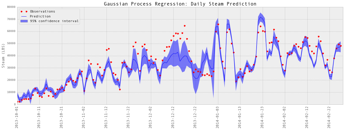
预测，计算精度和可视化

# Predict
gp, results_dailySteam = predictAll(0.1, 0.05, trainX_dailySteam, trainY_dailySteam,
                                    testX_dailySteam, testY_dailySteam, testSet_dailySteam, 'Daily Steam')
# Visualize
subset = results_dailySteam['2013-10':'2014-02']
testY = subset['steam-LBS']
predictedY = subset['predictedY']
sigma = subset['sigma']
plotGP(testY, predictedY, sigma)
plt.ylabel('Steam (LBS)', fontsize = 13)
plt.title('Gaussian Process Regression: Daily Steam Prediction', fontsize = 17)
plt.legend(loc='upper left')
plt.xlim([0, len(testY)])
#plt.ylim([1000,8000])
xTickLabels = pd.DataFrame(data = subset.index[np.arange(0,len(subset.index),10)],
                           columns=['datetime'])
xTickLabels['date'] = xTickLabels['datetime'].apply(lambda x: x.strftime('%Y-%m-%d'))
ax = plt.gca()
ax.set_xticks(np.arange(0, len(subset), 10))
ax.set_xticklabels(labels = xTickLabels['date'], fontsize = 13, rotation = 90)
plt.show()

Train score R2: 0.96729657748
Test score R2: 0.933120481633

以上是部分预测的可视化。

每小时的预测

我用同样的方法来训练和测试每小时的模型。因为随着数据点数量的增加，计算成本显著增加。在大型数据集上进行交叉验证是不可能的，因为我们没有太多的时间进行项目。因此，我只使用一小组训练/验证数据来获取参数，然后使用完整的数据集进行训练和测试，并让我的计算机连夜运行。

每小时用电量

获取训练/验证和测试集。先尝试小样本。dataframe显示特性和目标。

def addHourlyTimeFeatures(df):
    df['hour'] = df.index.hour
    df['weekday'] = df.index.weekday
    df['day'] = df.index.dayofyear
    df['week'] = df.index.weekofyear
    return df
hourlyElectricityWithFeatures = addHourlyTimeFeatures(hourlyElectricityWithFeatures)
df_hourlyElectricity = hourlyElectricityWithFeatures[['hour', 'weekday', 'day',
                                                      'week', 'cosHour',
                                                      'occupancy', 'electricity-kWh']]
#df_hourlyElectricity.to_excel('Data/trainSet_hourlyElectricity.xlsx')
def setTrainTestSets(df, trainStart, trainEnd, testStart, testEnd, indY):
    trainSet = df[trainStart : trainEnd]
    testSet = df[testStart : testEnd]
    trainX = trainSet.values[:,0:-1]
    trainY = trainSet.values[:,indY]
    testX = testSet.values[:,0:-1]
    testY = testSet.values[:,indY]
    return trainX, trainY, testX, testY, testSet
trainStart = '2013-02'
trainEnd = '2013-05'
testStart = '2014-03'
testEnd = '2014-04'
df = df_hourlyElectricity;
trainX_hourlyElectricity, trainY_hourlyElectricity, \
testX_hourlyElectricity, testY_hourlyElectricity, \
    testSet_hourlyElectricity = setTrainTestSets(df, trainStart,
                                                 trainEnd, testStart, testEnd, 6) 
df_hourlyElectricity.head()

	hour	weekday	day	week	cosHour	electricity-kWh
2012-01-01 01:00:00	1	6	1	52	0.866025	111.479277
2012-01-01 02:00:00	2	6	1	52	0.965926	117.989395
2012-01-01 03:00:00	3	6	1	52	1.000000	119.010131
2012-01-01 04:00:00	4	6	1	52	0.965926	116.005587
2012-01-01 05:00:00	5	6	1	52	0.866025	111.132977

交叉验证以获得输入参数

nugget = 0.008
theta = np.arange(0.05, 0.5, 0.05)
crossValidation(theta, nugget, 10, trainX_hourlyElectricity, trainY_hourlyElectricity)

预测，计算精度和可视化

gp_hourlyElectricity, results_hourlyElectricity = predictAll(0.1, 0.008,
                                                             trainX_hourlyElectricity,
                                                             trainY_hourlyElectricity,
                                                             testX_hourlyElectricity,
                                                             testY_hourlyElectricity,
                                                             testSet_hourlyElectricity,
                                                          'Hourly Electricity (Partial)')

Train score R2: 0.957912601164
Test score R2: 0.893873175566

subset = results_hourlyElectricity['2014-03-08 23:00:00':'2014-03-15']
testY = subset['electricity-kWh']
predictedY = subset['predictedY']
sigma = subset['sigma']
plotGP(testY, predictedY, sigma)
plt.ylabel('Electricity (kWh)', fontsize = 13)
plt.title('Gaussian Process Regression: Hourly Electricity Prediction', fontsize = 17)
plt.legend(loc='upper right')
plt.xlim([0, len(testY)])
#plt.ylim([1000,8000])
xTickLabels = subset.index[np.arange(0,len(subset.index),6)]
ax = plt.gca()
ax.set_xticks(np.arange(0, len(subset), 6))
ax.set_xticklabels(labels = xTickLabels, fontsize = 13, rotation = 90)
plt.show()

以上是部分预测的可视化。

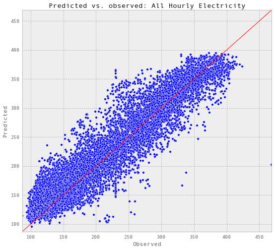
训练和测试每小时的数据

每小时电量的最终预测精度。

trainStart = '2012-01'
trainEnd = '2013-06'
testStart = '2013-07'
testEnd = '2014-10'
results_allHourlyElectricity = pd.read_excel('Data/results_allHourlyElectricity.xlsx')
def plotR2(df, energyType, title):
    testY = df[energyType]
    predictedY = df['predictedY']
    print "Test score R2:", sklearn.metrics.r2_score(testY, predictedY)
    plt.figure(figsize = (9,8))
    plt.scatter(testY, predictedY)
    plt.plot([min(testY), max(testY)], [min(testY), max(testY)], 'r')
    plt.xlim([min(testY), max(testY)])
    plt.ylim([min(testY), max(testY)])
    plt.title('Predicted vs. observed: ' + title)
    plt.xlabel('Observed')
    plt.ylabel('Predicted')
    plt.show()
plotR2(results_allHourlyElectricity, 'electricity-kWh', 'All Hourly Electricity')

Test score R2: 0.882986662109

每小时用冷水

获取训练/验证和测试集。先尝试小样本。dataframe显示特性和目标。

trainStart = '2013-08'
trainEnd = '2013-10'
testStart = '2014-08'
testEnd = '2014-10'
def getPredictedElectricity(trainStart, trainEnd, testStart, testEnd):
    trainX, trainY, testX, testY, testSet = setTrainTestSets(df_hourlyElectricity,
                                                             trainStart, trainEnd,
                                                             testStart, testEnd, 6) 
    gp = gaussian_process.GaussianProcess(theta0 = 0.15, nugget = 0.008)
    gp.fit(trainX, trainY)
    trainSet = df_hourlyElectricity[trainStart : trainEnd]
    predictedElectricity = pd.DataFrame(data = np.zeros(len(trainSet)),
                                        index = trainSet.index,
                                        columns = ['predictedElectricity'])
    predictedElectricity = \
    predictedElectricity.append(pd.DataFrame(data = np.zeros(len(testSet)),
                                             index = testSet.index,
                                             columns = ['predictedElectricity']))
    predictedElectricity.loc[trainStart:trainEnd,
                             'predictedElectricity'] = gp.predict(trainX)
    predictedElectricity.loc[testStart:testEnd,
                             'predictedElectricity'] = gp.predict(testX)
    return predictedElectricity
predictedElectricity = getPredictedElectricity(trainStart, trainEnd, testStart, testEnd)
hourlyChilledWaterWithMoreFeatures = \ hourlyChilledWaterWithFeatures.join(predictedElectricity, how = 'inner')
hourlyChilledWaterWithMoreFeatures = addHourlyTimeFeatures(hourlyChilledWaterWithMoreFeatures)
df_hourlyChilledWater = hourlyChilledWaterWithMoreFeatures[['hour', 'cosHour',
                                                            'weekday', 'day', 'week',
                                                            'occupancy', 'T-C',
                                                        	'humidityRatio-kg/kg',
                                                            'predictedElectricity',
                                                            'chilledWater-TonDays']]
df = df_hourlyChilledWater;
trainX_hourlyChilledWater, \
trainY_hourlyChilledWater, \
testX_hourlyChilledWater,  \
testY_hourlyChilledWater, \
testSet_hourlyChilledWater = setTrainTestSets(df, trainStart, trainEnd,
                                              testStart, testEnd, 9) 
df_hourlyChilledWater.head()

	hour	cosHour	weekday	day	week	occupancy	T-C	humidityRatio-kg/kg	predictedElectricity	chilledWater-TonDays
2013-08-01 00:00:00	0	0.707107	3	213	31	0.5	17.7	0.010765	123.431454	0.200647
2013-08-01 01:00:00	1	0.866025	3	213	31	0.5	17.8	0.012102	119.266616	0.183318
2013-08-01 02:00:00	2	0.965926	3	213	31	0.5	17.7	0.012026	121.821887	0.183318
2013-08-01 03:00:00	3	1.000000	3	213	31	0.5	17.6	0.011962	124.888675	0.183318
2013-08-01 04:00:00	4	0.965926	3	213	31	0.5	17.7	0.011912	124.824413	0.183318

交叉验证以获得输入参数

nugget = 0.01
theta = np.arange(0.001, 0.05, 0.01)
crossValidation(theta, nugget, 5, trainX_hourlyChilledWater, trainY_hourlyChilledWater)

预测，计算精度和可视化

gp_hourlyChilledWater, results_hourlyChilledWater = predictAll(0.011, 0.01,
                                                               trainX_hourlyChilledWater,
                                                               trainY_hourlyChilledWater,
                                                               testX_hourlyChilledWater,
                                                               testY_hourlyChilledWater,
                                                              testSet_hourlyChilledWater,
                                                      'Hourly Chilled Water (Particial)')

Train score R2: 0.914352370778
Test score R2: 0.865202975683

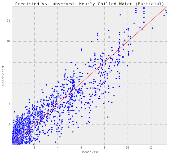
subset = results_hourlyChilledWater['2014-08-24':'2014-08-30']
testY = subset['chilledWater-TonDays']
predictedY = subset['predictedY']
sigma = subset['sigma']
plotGP(testY, predictedY, sigma)
plt.ylabel('Chilled water (ton-days)', fontsize = 13)
plt.title('Gaussian Process Regression: Hourly Chilled Water Prediction', fontsize = 17)
plt.legend(loc='upper right')
plt.xlim([0, len(testY)])
#plt.ylim([1000,8000])
xTickLabels = subset.index[np.arange(0,len(subset.index),6)]
ax = plt.gca()
ax.set_xticks(np.arange(0, len(subset), 6))
ax.set_xticklabels(labels = xTickLabels, fontsize = 13, rotation = 90)
plt.show()

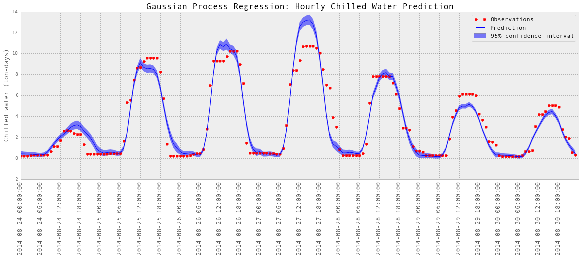
以上是部分预测的可视化。

训练和测试每小时的数据

警告:这可能需要很长时间才能执行代码。

# This could take forever.
trainStart = '2012-01'
trainEnd = '2013-06'
testStart = '2013-07'
testEnd = '2014-10'
predictedElectricity = getPredictedElectricity(trainStart, trainEnd, testStart, testEnd)
# Chilled water
hourlyChilledWaterWithMoreFeatures = hourlyChilledWaterWithFeatures.join(predictedElectricity, how = 'inner')
hourlyChilledWaterWithMoreFeatures = addHourlyTimeFeatures(hourlyChilledWaterWithMoreFeatures)
df_hourlyChilledWater = hourlyChilledWaterWithMoreFeatures[['hour', 'cosHour',
                                                            'weekday', 'day',
                                                            'week', 'occupancy', 'T-C',
                                                        	'humidityRatio-kg/kg',
                                                            'predictedElectricity',
                                                            'chilledWater-TonDays']]
df = df_hourlyChilledWater;
trainX_hourlyChilledWater, \
trainY_hourlyChilledWater, \
testX_hourlyChilledWater, \
testY_hourlyChilledWater, \
testSet_hourlyChilledWater = setTrainTestSets(df, trainStart, trainEnd,
                                              testStart, testEnd, 9) 
gp_hourlyChilledWater, results_hourlyChilledWater = predictAll(0.011, 0.01,
                                                               trainX_hourlyChilledWater,
                                                               trainY_hourlyChilledWater,
                                                               testX_hourlyChilledWater,
                                                               testY_hourlyChilledWater,
                                                              testSet_hourlyChilledWater)
results_hourlyChilledWater.to_excel('Data/results_allHourlyChilledWater.xlsx')

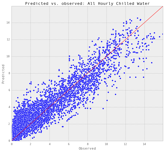
每小时冷水预报的最终精度。

results_allHourlyChilledWater = pd.read_excel('Data/results_allHourlyChilledWater.xlsx')
plotR2(results_allHourlyChilledWater, 'chilledWater-TonDays', 'All Hourly Chilled Water')

Test score R2: 0.887195665411

每小时用热水

获取训练/验证和测试集。先尝试小样本。dataframe显示特性和目标。

trainStart = '2012-01'
trainEnd = '2012-03'
testStart = '2014-01'
testEnd = '2014-03'    
predictedElectricity = getPredictedElectricity(trainStart, trainEnd, testStart, testEnd)
hourlySteamWithMoreFeatures = hourlySteamWithFeatures.join(predictedElectricity,
                                                           how = 'inner')
hourlySteamWithMoreFeatures = addHourlyTimeFeatures(hourlySteamWithMoreFeatures)
df_hourlySteam = hourlySteamWithMoreFeatures[['hour', 'cosHour', 'weekday',
                                              'day', 'week', 'occupancy', 'T-C',
                                              'humidityRatio-kg/kg',
                                              'predictedElectricity', 'steam-LBS']]
df = df_hourlySteam;
trainX_hourlySteam,
trainY_hourlySteam,
testX_hourlySteam,
testY_hourlySteam, \
testSet_hourlySteam = setTrainTestSets(df, trainStart, trainEnd, testStart, testEnd, 9) 
df_hourlySteam.head()

	hour	cosHour	weekday	day	week	T-C	humidityRatio-kg/kg	predictedElectricity	steam-LBS
2012-01-01 01:00:00	1	0.866025	6	1	52	4	0.004396	117.502720	513.102214
2012-01-01 02:00:00	2	0.965926	6	1	52	4	0.004391	114.720226	1353.371311
2012-01-01 03:00:00	3	1.000000	6	1	52	5	0.004380	113.079503	1494.904514
2012-01-01 04:00:00	4	0.965926	6	1	52	6	0.004401	112.428146	490.090061
2012-01-01 05:00:00	5	0.866025	6	1	52	4	0.004382	113.892620	473.258464

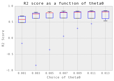
交叉验证以获得输入参数

nugget = 0.01
theta = np.arange(0.001, 0.014, 0.002)
crossValidation(theta, nugget, 5, trainX_hourlySteam, trainY_hourlySteam)

训练和测试每小时的数据

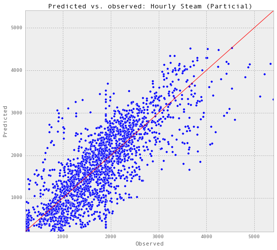
gp_hourlySteam, results_hourlySteam = predictAll(0.007, 0.01,
                                                 trainX_hourlySteam, trainY_hourlySteam,
                                  				 testX_hourlySteam, testY_hourlySteam, testSet_hourlySteam, 'Hourly Steam (Particial)')

Train score R2: 0.844826486064
Test score R2: 0.570427290315

subset = results_hourlySteam['2014-01-26':'2014-02-01']
testY = subset['steam-LBS']
predictedY = subset['predictedY']
sigma = subset['sigma']
plotGP(testY, predictedY, sigma)
plt.ylabel('Steam (LBS)', fontsize = 13)
plt.title('Gaussian Process Regression: Hourly Steam Prediction', fontsize = 17)
plt.legend(loc='upper right')
plt.xlim([0, len(testY)])
xTickLabels = subset.index[np.arange(0,len(subset.index),6)]
ax = plt.gca()
ax.set_xticks(np.arange(0, len(subset), 6))
ax.set_xticklabels(labels = xTickLabels, fontsize = 13, rotation = 90)
plt.show()

以上是部分预测的可视化。

尝试训练和测试每小时的热水

警告:这可能需要很长时间才能执行代码。

# Warning: this could take forever to execute the code.
trainStart = '2012-01'
trainEnd = '2013-06'
testStart = '2013-07'
testEnd = '2014-10'
predictedElectricity = getPredictedElectricity(trainStart, trainEnd, testStart, testEnd)
# Steam
hourlySteamWithMoreFeatures = hourlySteamWithFeatures.join(predictedElectricity,
                                                           how = 'inner')
hourlySteamWithMoreFeatures = addHourlyTimeFeatures(hourlySteamWithMoreFeatures)
df_hourlySteam = hourlySteamWithMoreFeatures[['hour', 'cosHour', 'weekday',
                                              'day', 'week', 'occupancy', 'T-C',
                                              'humidityRatio-kg/kg',
                                              'predictedElectricity', 'steam-LBS']]
df = df_hourlySteam;
trainX_hourlySteam, trainY_hourlySteam, testX_hourlySteam, testY_hourlySteam, \
    testSet_hourlySteam = setTrainTestSets(df, trainStart, trainEnd,
                                           testStart, testEnd, 9) 
gp_hourlySteam, results_hourlySteam = predictAll(0.007, 0.01,
                                                 trainX_hourlySteam, trainY_hourlySteam,
                                                 testX_hourlySteam, testY_hourlySteam,
                                                 testSet_hourlySteam)
results_hourlySteam.to_excel('Data/results_allHourlySteam.xlsx')

Final accuracy for hourly steam prediction.

results_allHourlySteam = pd.read_excel('Data/results_allHourlySteam.xlsx')
plotR2(results_allHourlySteam, 'steam-LBS', 'All Hourly Steam')

Test score R2: 0.84405417838

每小时的预测不如每天的好。但是R2的值仍然是0.85。

总结

高斯过程回归的整体性能非常好。GP的优点是提供了预测的不确定范围。缺点是对于大型数据集来说，它的计算开销非常大。

下篇4_Random Forests and K-Nearest Neighbours

翻译——3_Gaussian Process Regression的更多相关文章

翻译——2_Linear Regression and Support Vector Regression
续上篇 1_Project Overview, Data Wrangling and Exploratory Analysis 使用不同的机器学习方法进行预测线性回归在这本笔记本中,将训练一个线性 ...
Scalaz（50）－ scalaz-stream: 安全的无穷运算－running infinite stream freely
scalaz-stream支持无穷数据流(infinite stream),这本身是它强大的功能之一,试想有多少系统需要通过无穷运算才能得以实现.这是因为外界的输入是不可预料的,对于系统本身就是无穷的 ...
The Model Complexity Myth
The Model Complexity Myth (or, Yes You Can Fit Models With More Parameters Than Data Points) An oft- ...
Summary on Visual Tracking: Paper List, Benchmarks and Top Groups
Summary on Visual Tracking: Paper List, Benchmarks and Top Groups 2018-07-26 10:32:15 This blog is c ...
机器学习理论基础学习18---高斯过程回归(GPR)
一.高斯(分布)过程(随机过程)是什么? 一维高斯分布多维高斯分布无限维高斯分布高斯网络高斯过程简单的说,就是一系列关于连续域(时间或空间)的随机变量的联合,而且针对每一个时间或是空间点 ...
Resources in Visual Tracking
这个应该是目前最全的Tracking相关的文章了一.Surveyand benchmark: 1. PAMI2014:VisualTracking_ An Experimental Sur ...
ECCV 2014 Results (16 Jun, 2014) 结果已出
Accepted Papers Title Primary Subject Area ID 3D computer vision 93 UPnP: An optimal O(n) soluti ...
CVPR 2015 papers
CVPR2015 Papers震撼来袭! CVPR 2015的文章可以下载了,如果链接无法下载,可以在Google上通过搜索paper名字下载(友情提示:可以使用filetype:pdf命令). Go ...
nodejs api 中文文档
文档首页英文版文档本作品采用知识共享署名-非商业性使用 3.0 未本地化版本许可协议进行许可. Node.js v0.10.18 手册 & 文档索引 | 在单一页面中浏览 | JSON格 ...

随机推荐

015、MySQL取今天是第几季度，往后几个月是第几季度
#取今天是第几季度 SELECT QUARTER( curdate( ) ); #取往后几个月是第几季度 , INTERVAL MONTH ) ); , INTERVAL MONTH ) ); , I ...
ios端简单改变webView的黑白夜模式
extension HTController:WKUIDelegate, WKNavigationDelegate,WKScriptMessageHandler { func userContentC ...
【LOJ6498】「雅礼集训 2018 Day2」农民
题面 solution 直接暴力模拟,原数据可获得满分的成绩. 对于每个点,其父亲对其都有一个限制.故我们只需要判断当前点到根的路径上的限制是否都能满足即可. 考虑用树剖+线段树维护这个限制.考虑到翻 ...
CharacterEncodingFilter详解及源码解析
字符编码过滤器 (Spring框架对字符编码的处理) 基于函数回调,对所有请求起作用,只在容器初始化时调用一次,依赖于servlet容器. web.xml配置文件 <filter> &l ...
E. MaratonIME does (not do) PAs
E. MaratonIME does (not do) PAs time limit per test 2.0 s memory limit per test 256 MB input standar ...
3分钟教你用python制作一个简单词云
首先需要安装三个包: # 安装:pip install matplotlib # 安装:pip install jieba # 安装pip install wordcloud 1.制作英文字母的词云 ...
servlet中调用注入spring管理的dao（转）
今天做大型仪器的的时候遇到的问题,转下为了以后能用 http://blog.csdn.net/jiyingying_up/article/details/44803585 我们用spring的依赖注入 ...
Codeforces Round #585 (Div. 2) CF1215A~C
CF1215A. Yellow Cards简单的模拟,给定了黄票张数,判断最少和最多有多少人被罚下场. #include <bits/stdc++.h> using namespace s ...
SMPL模型Shape和Pose参数
两部分 1.Pose参数 2.Shape参数一 Pose参数共24个关节点,对应idx从0到23,图中3个小图分别表示zero shape只有idx节点分别绕x/y/z轴旋转. 其中蓝色线表示-p ...
部署Ambari Server实战案例
部署Ambari Server实战案例作者:尹正杰版权声明:原创作品,谢绝转载!否则将追究法律责任. 一.准备三台虚拟机(需要自行安装jdk环境) 1>.角色分配 NameNode节点: h ...

翻译——3_Gaussian Process Regression

使用不同的机器学习方法进行预测

高斯过程回归

每日预测:

每日用电

每日冷水

再增加一个特性:电量预测

热水

每小时的预测

每小时用电量

训练和测试每小时的数据

每小时用冷水

训练和测试每小时的数据

每小时用热水

尝试训练和测试每小时的热水

总结

翻译——3_Gaussian Process Regression的更多相关文章

随机推荐

热门专题