课程一(Neural Networks and Deep Learning)，第四周（Deep Neural Networks） —— 3.Programming Assignments: Deep Neural Network - Application

Deep Neural Network - Application

Congratulations! Welcome to the fourth programming exercise of the deep learning specialization. You will now use everything you have learned to build a deep neural network that classifies cat vs. non-cat images.

　　　　　　　　　　　　　　

In the second exercise, you used logistic regression to build cat vs. non-cat images and got a 68% accuracy. Your algorithm will now give you an 80% accuracy! By completing this assignment, you will:

　　- Learn how to use all the helper functions you built in the previous assignment to build a model of any structure you want.

　　- Experiment with different model architectures and see how each one behaves.

　　- Recognize that it is always easier to build your helper functions before attempting to build a neural network from scratch.

This assignment prepares you well for the next course which dives deep into the techniques and strategies for parameters tuning and initializations. Take your time to complete this assignment and make sure you get the expected outputs when working through the different exercises. In some code blocks, you will find a "#GRADED FUNCTION: functionName" comment. Please do not modify it. After you are done, submit your work and check your results. You need to score 70% to pass. Good luck :) !

【中文翻译】

深神经网络-应用

祝贺!欢迎来到深度学习专业第四次编程练习。现在你将使用你所学到的一切建立一个深层的神经网络, 将cat与 non-cat 的图像分类。

在第二个练习中, 您使用逻辑回归来构建 cat 与 non-cat 的图像, 并获得了68% 的准确性。你的算法现在将给你一个80% 的精确度!通过完成此任务, 您将:

　　-了解如何使用在上一个工作分配中生成的所有帮助器函数来构建所需的任何结构的模型。

　　-尝试使用不同的模型体系结构, 并查看每种架构的效果。

　　-认识到, 在尝试从头构建神经网络之前, 构建帮助函数总是比较容易的。

这项任务为您下一课做好了准备。下一课将 深入了解参数调整和初始化的技术和策略。用你的时间完成这个任务, 通过不同的练习，并确保你得到预期的结果 。在某些代码块中, 您将找到一个 "#GRADED FUNCTION: functionName" 的注释。请不要修改它。完成后, 提交您的工作, 并检查您的结果。你需要得分70% 才能过关。祝你好运:)!

-------------------------------------------------------------------------------------------------

Deep Neural Network for Image Classification: Application

When you finish this, you will have finished the last programming assignment of Week 4, and also the last programming assignment of this course!

You will use use the functions you'd implemented in the previous assignment to build a deep network, and apply it to cat vs non-cat classification. Hopefully, you will see an improvement in accuracy relative to your previous logistic regression implementation.

After this assignment you will be able to:

• Build and apply a deep neural network to supervised learning.

Let's get started!

1 - Packages

Let's first import all the packages that you will need during this assignment.

• numpy is the fundamental package for scientific computing with Python.
• matplotlib is a library to plot graphs in Python.
• h5py is a common package to interact with a dataset that is stored on an H5 file.
• PIL and scipy are used here to test your model with your own picture at the end.
• dnn_app_utils provides the functions implemented in the "Building your Deep Neural Network: Step by Step" assignment to this notebook.
• np.random.seed(1) is used to keep all the random function calls consistent. It will help us grade your work.

【code】

import time
import numpy as np
import h5py
import matplotlib.pyplot as plt
import scipy
from PIL import Image
from scipy import ndimage
from dnn_app_utils_v2 import *

%matplotlib inline
plt.rcParams['figure.figsize'] = (5.0, 4.0) # set default size of plots
plt.rcParams['image.interpolation'] = 'nearest'
plt.rcParams['image.cmap'] = 'gray'

%load_ext autoreload
%autoreload 2

np.random.seed(1)

-------------------------------------------------------------------------------------------------

2 - Dataset

You will use the same "Cat vs non-Cat" dataset as in "Logistic Regression as a Neural Network" (Assignment 2). The model you had built had 70% test accuracy on classifying cats vs non-cats images. Hopefully, your new model will perform a better!

Problem Statement: You are given a dataset ("data.h5") containing:

- a training set of m_train images labelled as cat (1) or non-cat (0)
- a test set of m_test images labelled as cat and non-cat
- each image is of shape (num_px, num_px, 3) where 3 is for the 3 channels (RGB).

Let's get more familiar with the dataset. Load the data by running the cell below.

train_x_orig, train_y, test_x_orig, test_y, classes = load_data()

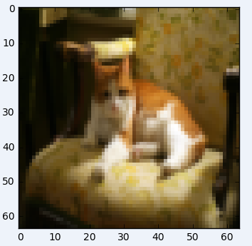
The following code will show you an image in the dataset. Feel free to change the index and re-run the cell multiple times to see other images.

# Example of a picture
index = 7
plt.imshow(train_x_orig[index])
print ("y = " + str(train_y[0,index]) + ". It's a " + classes[train_y[0,index]].decode("utf-8") +  " picture.")

y = 1. It's a cat picture.

【code】

# Explore your dataset
m_train = train_x_orig.shape[0] # 行数
num_px = train_x_orig.shape[1]  # 列数
m_test = test_x_orig.shape[0]  # 行数

print ("Number of training examples: " + str(m_train))
print ("Number of testing examples: " + str(m_test))
print ("Each image is of size: (" + str(num_px) + ", " + str(num_px) + ", 3)")
print ("train_x_orig shape: " + str(train_x_orig.shape))
print ("train_y shape: " + str(train_y.shape))
print ("test_x_orig shape: " + str(test_x_orig.shape))
print ("test_y shape: " + str(test_y.shape))

【result】

Number of training examples: 209
Number of testing examples: 50
Each image is of size: (64, 64, 3)
train_x_orig shape: (209, 64, 64, 3)
train_y shape: (1, 209)
test_x_orig shape: (50, 64, 64, 3)
test_y shape: (1, 50)

As usual, you reshape and standardize the images before feeding them to the network. The code is given in the cell below.

【code】

# Reshape the training and test examples
train_x_flatten = train_x_orig.reshape(train_x_orig.shape[0], -1).T   # The "-1" makes reshape flatten the remaining dimensions
test_x_flatten = test_x_orig.reshape(test_x_orig.shape[0], -1).T  #  "-1" 使得剩下的维度变为1维

# Standardize data to have feature values between 0 and 1.
train_x = train_x_flatten/255.
test_x = test_x_flatten/255.

print ("train_x's shape: " + str(train_x.shape))
print ("test_x's shape: " + str(test_x.shape))

【result】

train_x's shape: (12288, 209)
test_x's shape: (12288, 50)

12,288equals 64×64×3 which is the size of one reshaped image vector.

-------------------------------------------------------------------------------------------------

 

3 - Architecture of your model

Now that you are familiar with the dataset, it is time to build a deep neural network to distinguish cat images from non-cat images.

You will build two different models:

• A 2-layer neural network
• An L-layer deep neural network

You will then compare the performance of these models, and also try out different values for LL.

Let's look at the two architectures.

3.1 - 2-layer neural network

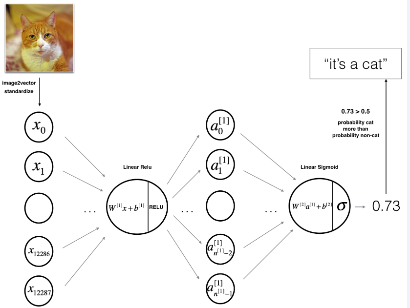
　　　　　　　　　　　　　　　　　　Figure 2: 2-layer neural network. 
　　　　　　The model can be summarized as: INPUT -> LINEAR -> RELU -> LINEAR -> SIGMOID -> OUTPUT.

Detailed Architecture of figure 2:

• The input is a (64,64,3) image which is flattened to a vector of size (12288,1).
• The corresponding vector: [x₀,x₁,...,x₁₂₂₈₇]^Tis then multiplied by the weight matrix W^[1]of size (n^[1],12288).
• You then add a bias term and take its relu to get the following vector: [a₀^[1],a₁^[1],...,an_[1]−1^[1]]^T
• You then repeat the same process.
• You multiply the resulting vector by W^[2]and add your intercept (bias).            # intercept ：截距
• Finally, you take the sigmoid of the result. If it is greater than 0.5, you classify it to be a cat.

3.2 - L-layer deep neural network

It is hard to represent an L-layer deep neural network with the above representation. However, here is a simplified network representation:

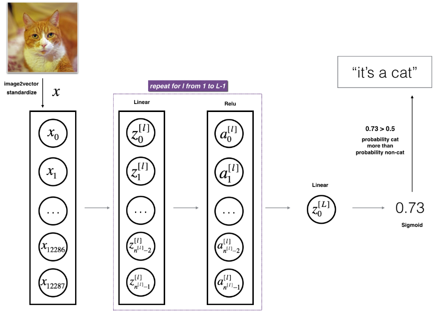
　　　　　　　　　　　　　　Figure 3: L-layer neural network. 
　　　　　　The model can be summarized as: [LINEAR -> RELU] × (L-1) -> LINEAR -> SIGMOID

Detailed Architecture of figure 3:

• The input is a (64,64,3) image which is flattened to a vector of size (12288,1).
• The corresponding vector:  [x₀,x₁,...,x₁₂₂₈₇]^T is then multiplied by the weight matrix W^[1] and then you add the intercept b^[1]. The result is called the linear unit.
• Next, you take the relu of the linear unit. This process could be repeated several times for each (W^[l],b[^l])depending on the model architecture.
• Finally, you take the sigmoid of the final linear unit. If it is greater than 0.5, you classify it to be a cat.

3.3 - General methodology

As usual you will follow the Deep Learning methodology to build the model:

1. Initialize parameters / Define hyperparameters
2. Loop for num_iterations:
    a. Forward propagation
    b. Compute cost function
    c. Backward propagation
    d. Update parameters (using parameters, and grads from backprop)
4. Use trained parameters to predict labels

Let's now implement those two models!

-------------------------------------------------------------------------------------------------

4 - Two-layer neural network

Question: Use the helper functions you have implemented in the previous assignment to build a 2-layer neural network with the following structure: LINEAR -> RELU -> LINEAR -> SIGMOID. The functions you may need and their inputs are:

def initialize_parameters(n_x, n_h, n_y):
    ...
    return parameters
def linear_activation_forward(A_prev, W, b, activation):
    ...
    return A, cache
def compute_cost(AL, Y):
    ...
    return cost
def linear_activation_backward(dA, cache, activation):
    ...
    return dA_prev, dW, db
def update_parameters(parameters, grads, learning_rate):
    ...
    return parameters

【code】

### CONSTANTS DEFINING THE MODEL ####
n_x = 12288     # num_px * num_px * 3
n_h = 7
n_y = 1
layers_dims = (n_x, n_h, n_y)

# GRADED FUNCTION: two_layer_model

def two_layer_model(X, Y, layers_dims, learning_rate = 0.0075, num_iterations = 3000, print_cost=False):
    """
    Implements a two-layer neural network: LINEAR->RELU->LINEAR->SIGMOID.

    Arguments:
    X -- input data, of shape (n_x, number of examples)
    Y -- true "label" vector (containing 0 if cat, 1 if non-cat), of shape (1, number of examples)
    layers_dims -- dimensions of the layers (n_x, n_h, n_y)
    num_iterations -- number of iterations of the optimization loop
    learning_rate -- learning rate of the gradient descent update rule
    print_cost -- If set to True, this will print the cost every 100 iterations 

    Returns:
    parameters -- a dictionary containing W1, W2, b1, and b2
    """

    np.random.seed(1)
    grads = {}
    costs = []                              # to keep track of the cost
    m = X.shape[1]                           # number of examples
    (n_x, n_h, n_y) = layers_dims

    # Initialize parameters dictionary, by calling one of the functions you'd previously implemented
    ### START CODE HERE ### (≈ 1 line of code)
    parameters = initialize_parameters(n_x, n_h, n_y)
    ### END CODE HERE ###

    # Get W1, b1, W2 and b2 from the dictionary parameters.
    W1 = parameters["W1"]
    b1 = parameters["b1"]
    W2 = parameters["W2"]
    b2 = parameters["b2"]

    # Loop (gradient descent)

    for i in range(0, num_iterations):

        # Forward propagation: LINEAR -> RELU -> LINEAR -> SIGMOID. Inputs: "X, W1, b1". Output: "A1, cache1, A2, cache2".
        ### START CODE HERE ### (≈ 2 lines of code)
        A1, cache1 = linear_activation_forward(X, W1, b1, activation = "relu")
        A2, cache2 = linear_activation_forward(A1, W2, b2, activation = "sigmoid")
        ### END CODE HERE ###

        # Compute cost
        ### START CODE HERE ### (≈ 1 line of code)
        cost = compute_cost(A2, Y)
        ### END CODE HERE ###

        # Initializing backward propagation
        dA2 = - (np.divide(Y, A2) - np.divide(1 - Y, 1 - A2))

        # Backward propagation. Inputs: "dA2, cache2, cache1". Outputs: "dA1, dW2, db2; also dA0 (not used), dW1, db1".
        ### START CODE HERE ### (≈ 2 lines of code)
        dA1, dW2, db2 = linear_activation_backward(dA2, cache2, activation = "sigmoid")
        dA0, dW1, db1 = linear_activation_backward(dA1, cache1, activation = "relu")
        ### END CODE HERE ###

        # Set grads['dWl'] to dW1, grads['db1'] to db1, grads['dW2'] to dW2, grads['db2'] to db2
        grads['dW1'] = dW1
        grads['db1'] = db1
        grads['dW2'] = dW2
        grads['db2'] = db2

        # Update parameters.
        ### START CODE HERE ### (approx. 1 line of code)
        parameters = update_parameters(parameters, grads, learning_rate)
        ### END CODE HERE ###

        # Retrieve W1, b1, W2, b2 from parameters
        W1 = parameters["W1"]
        b1 = parameters["b1"]
        W2 = parameters["W2"]
        b2 = parameters["b2"]

        # Print the cost every 100 training example
        if print_cost and i % 100 == 0:
            print("Cost after iteration {}: {}".format(i, np.squeeze(cost)))
        if print_cost and i % 100 == 0:
            costs.append(cost)

    # plot the cost

    plt.plot(np.squeeze(costs))
    plt.ylabel('cost')
    plt.xlabel('iterations (per tens)')
    plt.title("Learning rate =" + str(learning_rate))
    plt.show()

    return parameters

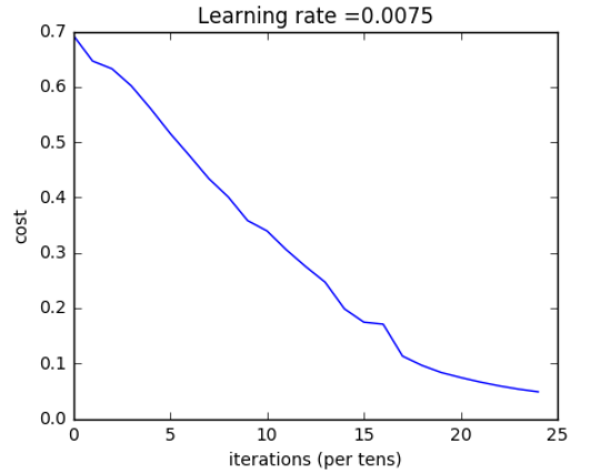
Run the cell below to train your parameters. See if your model runs. The cost should be decreasing. It may take up to 5 minutes to run 2500 iterations. Check if the "Cost after iteration 0" matches the expected output below, if not click on the square (⬛) on the upper bar of the notebook to stop the cell and try to find your error.

【code】

parameters = two_layer_model(train_x, train_y, layers_dims = (n_x, n_h, n_y), num_iterations = 2500, print_cost=True)

【result】

Cost after iteration 0: 0.693049735659989
Cost after iteration 100: 0.6464320953428849
Cost after iteration 200: 0.6325140647912678
Cost after iteration 300: 0.6015024920354665
Cost after iteration 400: 0.5601966311605748
Cost after iteration 500: 0.515830477276473
Cost after iteration 600: 0.4754901313943325
Cost after iteration 700: 0.43391631512257495
Cost after iteration 800: 0.4007977536203886
Cost after iteration 900: 0.35807050113237987
Cost after iteration 1000: 0.3394281538366413
Cost after iteration 1100: 0.30527536361962654
Cost after iteration 1200: 0.2749137728213015
Cost after iteration 1300: 0.24681768210614827
Cost after iteration 1400: 0.1985073503746611
Cost after iteration 1500: 0.17448318112556593
Cost after iteration 1600: 0.1708076297809661
Cost after iteration 1700: 0.11306524562164737
Cost after iteration 1800: 0.09629426845937163
Cost after iteration 1900: 0.08342617959726878
Cost after iteration 2000: 0.0743907870431909
Cost after iteration 2100: 0.06630748132267938
Cost after iteration 2200: 0.05919329501038176
Cost after iteration 2300: 0.05336140348560564
Cost after iteration 2400: 0.048554785628770226

Expected Output:

Cost after iteration 0	0.6930497356599888
Cost after iteration 100	0.6464320953428849
...	...
Cost after iteration 2400	0.048554785628770206

Good thing you built a vectorized implementation! Otherwise it might have taken 10 times longer to train this.

Now, you can use the trained parameters to classify images from the dataset. To see your predictions on the training and test sets, run the cell below.

【code】

predictions_train = predict(train_x, train_y, parameters)

【result】

Accuracy: 1.0

Expected Output:

Accuracy

1.0

 

【code】

predictions_test = predict(test_x, test_y, parameters)

【result】

Accuracy: 0.72

Expected Output:

Accuracy

0.72

 

Note: You may notice that running the model on fewer iterations (say 1500) gives better accuracy on the test set. This is called "early stopping" and we will talk about it in the next course. Early stopping is a way to prevent overfitting.

Congratulations! It seems that your 2-layer neural network has better performance (72%) than the logistic regression implementation (70%, assignment week 2). Let's see if you can do even better with an LL-layer model.

-------------------------------------------------------------------------------------------------

5 - L-layer Neural Network

Question: Use the helper functions you have implemented previously to build an LL-layer neural network with the following structure: [LINEAR -> RELU]×(L-1) -> LINEAR -> SIGMOID. The functions you may need and their inputs are:

def initialize_parameters_deep(layer_dims):
    ...
    return parameters
def L_model_forward(X, parameters):
    ...
    return AL, caches
def compute_cost(AL, Y):
    ...
    return cost
def L_model_backward(AL, Y, caches):
    ...
    return grads
def update_parameters(parameters, grads, learning_rate):
    ...
    return parameters

【code】

### CONSTANTS ###
layers_dims = [12288, 20, 7, 5, 1] #  5-layer model

【code】

# GRADED FUNCTION: L_layer_model

def L_layer_model(X, Y, layers_dims, learning_rate = 0.0075, num_iterations = 3000, print_cost=False):#lr was 0.009
    """
    Implements a L-layer neural network: [LINEAR->RELU]*(L-1)->LINEAR->SIGMOID.

    Arguments:
    X -- data, numpy array of shape (number of examples, num_px * num_px * 3)
    Y -- true "label" vector (containing 0 if cat, 1 if non-cat), of shape (1, number of examples)
    layers_dims -- list containing the input size and each layer size, of length (number of layers + 1).
    learning_rate -- learning rate of the gradient descent update rule
    num_iterations -- number of iterations of the optimization loop
    print_cost -- if True, it prints the cost every 100 steps

    Returns:
    parameters -- parameters learnt by the model. They can then be used to predict.
    """

    np.random.seed(1)
    costs = []                         # keep track of cost

    # Parameters initialization.
    ### START CODE HERE ###
    parameters = initialize_parameters_deep(layers_dims)
    ### END CODE HERE ###

    # Loop (gradient descent)
    for i in range(0, num_iterations):

        # Forward propagation: [LINEAR -> RELU]*(L-1) -> LINEAR -> SIGMOID.
        ### START CODE HERE ### (≈ 1 line of code)
        AL, caches =  L_model_forward(X, parameters)
        ### END CODE HERE ###

        # Compute cost.
        ### START CODE HERE ### (≈ 1 line of code)
        cost = compute_cost(AL, Y)
        ### END CODE HERE ###

        # Backward propagation.
        ### START CODE HERE ### (≈ 1 line of code)
        grads = L_model_backward(AL, Y, caches)
        ### END CODE HERE ###

        # Update parameters.
        ### START CODE HERE ### (≈ 1 line of code)
        parameters = update_parameters(parameters, grads, learning_rate)
        ### END CODE HERE ###

        # Print the cost every 100 training example
        if print_cost and i % 100 == 0:
            print ("Cost after iteration %i: %f" %(i, cost))
        if print_cost and i % 100 == 0:
            costs.append(cost)

    # plot the cost
    plt.plot(np.squeeze(costs))
    plt.ylabel('cost')
    plt.xlabel('iterations (per tens)')
    plt.title("Learning rate =" + str(learning_rate))
    plt.show()

    return parameters

You will now train the model as a 5-layer neural network.

Run the cell below to train your model. The cost should decrease on every iteration. It may take up to 5 minutes to run 2500 iterations. Check if the "Cost after iteration 0" matches the expected output below, if not click on the square (⬛) on the upper bar of the notebook to stop the cell and try to find your error.

【code】

parameters = L_layer_model(train_x, train_y, layers_dims, num_iterations = 2500, print_cost = True)

【result】

Cost after iteration 0: 0.771749
Cost after iteration 100: 0.672053
Cost after iteration 200: 0.648263
Cost after iteration 300: 0.611507
Cost after iteration 400: 0.567047
Cost after iteration 500: 0.540138
Cost after iteration 600: 0.527930
Cost after iteration 700: 0.465477
Cost after iteration 800: 0.369126
Cost after iteration 900: 0.391747
Cost after iteration 1000: 0.315187
Cost after iteration 1100: 0.272700
Cost after iteration 1200: 0.237419
Cost after iteration 1300: 0.199601
Cost after iteration 1400: 0.189263
Cost after iteration 1500: 0.161189
Cost after iteration 1600: 0.148214
Cost after iteration 1700: 0.137775
Cost after iteration 1800: 0.129740
Cost after iteration 1900: 0.121225
Cost after iteration 2000: 0.113821
Cost after iteration 2100: 0.107839
Cost after iteration 2200: 0.102855
Cost after iteration 2300: 0.100897
Cost after iteration 2400: 0.092878

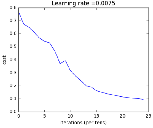
Expected Output:

Cost after iteration 0	0.771749
Cost after iteration 100	0.672053
...	...
Cost after iteration 2400	0.092878

 

 【code】

pred_train = predict(train_x, train_y, parameters)

【result】

Accuracy: 0.985645933014

Expected Output:

Train Accuracy

0.985645933014

【code】

pred_test = predict(test_x, test_y, parameters)

【result】

Accuracy: 0.8

Expected Output:

Test Accuracy

0.8

 

Congrats! It seems that your 5-layer neural network has better performance (80%) than your 2-layer neural network (72%) on the same test set.

This is good performance for this task. Nice job!

Though in the next course on "Improving deep neural networks" you will learn how to obtain even higher accuracy by systematically searching for better hyperparameters (learning_rate, layers_dims, num_iterations, and others you'll also learn in the next course).

-------------------------------------------------------------------------------------------------

6 Results Analysis

First, let's take a look at some images the L-layer model labeled incorrectly. This will show a few mislabeled images.

【code】

print_mislabeled_images(classes, test_x, test_y, pred_test)

【result】

 

A few type of images the model tends to do poorly on include:

• Cat body in an unusual position   猫身体在一个不寻常的位置
• Cat appears against a background of a similar color  猫在类似颜色的背景下出现
• Unusual cat color and species  不寻常的猫的颜色和种类
• Camera Angle  摄像机角度
• Brightness of the picture  图片的亮度
• Scale variation (cat is very large or small in image)  规模变化 (猫是非常大或小的图像)

-------------------------------------------------------------------------------------------------

7 Test with your own image (optional/ungraded exercise)

Congratulations on finishing this assignment. You can use your own image and see the output of your model. To do that:

1. Click on "File" in the upper bar of this notebook, then click "Open" to go on your Coursera Hub.
2. Add your image to this Jupyter Notebook's directory, in the "images" folder
3. Change your image's name in the following code
4. Run the code and check if the algorithm is right (1 = cat, 0 = non-cat)!

## START CODE HERE ##
my_image = "my_image.jpg" # change this to the name of your image file
my_label_y = [1] # the true class of your image (1 -> cat, 0 -> non-cat)
## END CODE HERE ##

fname = "images/" + my_image
image = np.array(ndimage.imread(fname, flatten=False))
my_image = scipy.misc.imresize(image, size=(num_px,num_px)).reshape((num_px*num_px*3,1))
my_predicted_image = predict(my_image, my_label_y, parameters)

plt.imshow(image)
print ("y = " + str(np.squeeze(my_predicted_image)) + ", your L-layer model predicts a \"" + classes[int(np.squeeze(my_predicted_image)),].decode("utf-8") +  "\" picture.")

【result】

Accuracy: 1.0
y = 1.0, your L-layer model predicts a "cat" picture.