《DSP using MATLAB》示例Example4.12

上代码：

b = [0, 1, 1]; a = [1, -0.9, 0.81];               %  

[R, p, C] = residuez(b,a);

Mp = (abs(p))'
Ap = (angle(p))'/pi

%% ----------------------------------------------
%%   START a    determine H(z) and sketch
%% ----------------------------------------------
figure('NumberTitle', 'off', 'Name', 'Example4.12 H(z) its pole-zero plot')
set(gcf,'Color','white');
zplane(b,a);
title('pole-zero plot'); grid on;

%% ----------------------------------------------
%%    END
%% ----------------------------------------------

%% --------------------------------------------------------------
%%    START    b   |H|   <H
%%    1st form of freqz
%% --------------------------------------------------------------
[H,w] = freqz(b,a,100);                 % 1st form of freqz

magH  = abs(H);  angH  = angle(H);  realH  = real(H);  imagH  = imag(H);

%% ================================================
%%              START H's  mag ang real imag
%% ================================================
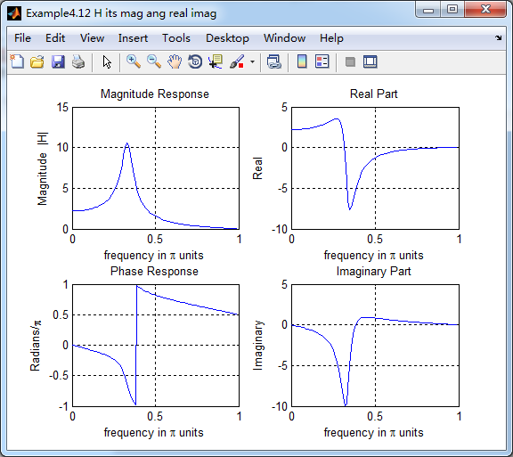
figure('NumberTitle', 'off', 'Name', 'Example4.12 H its mag ang real imag');
set(gcf,'Color','white');
subplot(2,2,1); plot(w/pi,magH); grid on;  %axis([0,1,0,1.5]);
title('Magnitude Response');
xlabel('frequency in \pi units'); ylabel('Magnitude  |H|');
subplot(2,2,3); plot(w/pi, angH/pi); grid on; % axis([-1,1,-1,1]);
title('Phase Response');
xlabel('frequency in \pi units'); ylabel('Radians/\pi');

subplot('2,2,2'); plot(w/pi, realH); grid on;
title('Real Part');
xlabel('frequency in \pi units'); ylabel('Real');
subplot('2,2,4'); plot(w/pi, imagH); grid on;
title('Imaginary Part');
xlabel('frequency in \pi units'); ylabel('Imaginary');
%% ==================================================
%%             END H's  mag ang real imag
%% ==================================================

%% ---------------------------------------------------------------
%%    END    b   |H|   <H
%% ---------------------------------------------------------------

%% --------------------------------------------------------------
%%    START    b   |H|   <H
%%    3rd form of freqz
%% --------------------------------------------------------------
w = [0:1:100]*pi/100;     H = freqz(b,a,w);
%[H,w] = freqz(b,a,200,'whole');                 % 3rd form of freqz

magH  = abs(H);  angH  = angle(H);  realH  = real(H);  imagH  = imag(H);

%% ================================================
%%              START H's  mag ang real imag
%% ================================================
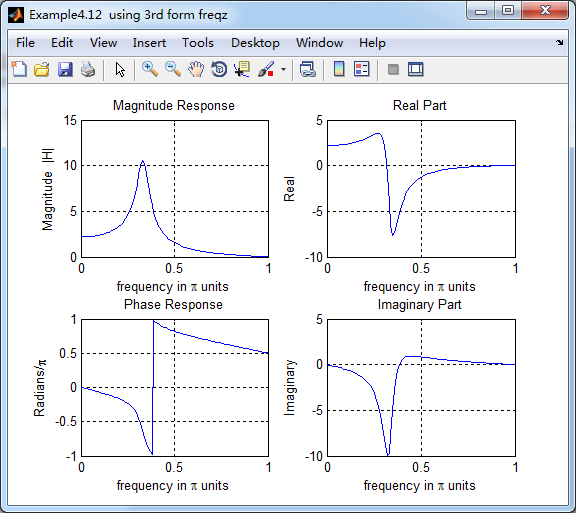
figure('NumberTitle', 'off', 'Name', 'Example4.12  using 3rd form freqz ');
set(gcf,'Color','white');
subplot(2,2,1); plot(w/pi,magH); grid on;  %axis([0,1,0,1.5]);
title('Magnitude Response');
xlabel('frequency in \pi units'); ylabel('Magnitude  |H|');
subplot(2,2,3); plot(w/pi, angH/pi); grid on; % axis([-1,1,-1,1]);
title('Phase Response');
xlabel('frequency in \pi units'); ylabel('Radians/\pi');

subplot('2,2,2'); plot(w/pi, realH); grid on;
title('Real Part');
xlabel('frequency in \pi units'); ylabel('Real');
subplot('2,2,4'); plot(w/pi, imagH); grid on;
title('Imaginary Part');
xlabel('frequency in \pi units'); ylabel('Imaginary');
%% ==================================================
%%             END H's  mag ang real imag
%% ==================================================

%% ---------------------------------------------------------------
%%    END    b   |H|   <H
%% ---------------------------------------------------------------

　　结果：