POMDP
本文转自:http://www.pomdp.org/
一、Background on POMDPs
We assume that the reader is familiar with the value iteration algorithm for regular discrete Markov decision processes (MDPs). However, we will need to differentiate these from POMDPs which we could also call a discrete Markov decision process. Therefore, we will refer to the more familiar MDPs as CO-MDPs, emphasizing that they are completely observable.
Adding partial observability to an MDP is not a trivial addition. Solution procedures for CO-MDPs give values or policies for each state. Use of these solutions requires the state to be completely known at all times and with complete observability this presents no problem. Partial observability clouds the idea of the current state. No longer is there certainty about the current state which makes selecting actions based on the current state (as in a CO-MDP) no longer valid.
A POMDP is really just an MDP; we have a set of states, a set of actions, transitions and immediate rewards. The actions' effects on the state in a POMDP is exactly the same as in an MDP. The only difference is in whether or not we can observe the current state of the process. In a POMDP we add a set of observations to the model. So instead of directly observing the current state, the state gives us an observation which provides a hint about what state it is in. The observations can be probabilistic; so we need to also specify an observation function. This observation function simply tells us the probability of each observation for each state in the model. We can also have the observation likelihood depend on the action if we like.
Although the underlying dynamics of the POMDP are still Markovian, since we have no direct access to the current state, our decisions require keeping track of (possibly) the entire history of the process, making this a non-Markovian process. The history at a given point in time is comprised of our knowledge about our starting situation, all actions performed and all observations seen.
Fortunately, it turns out that simply maintaining a probability distribution over all of the states provides us with the same information as if we maintained the complete history. In a CO-MDP we track our current state and update it after each action. Here this is trivial, because it is completely observable. In a POMDP we have to maintain this probability distribution over states. When we perform and action and make an observation, we have to update the distribution. Updating the distribution is very easy and just involves using the transition and observation probabilities. You'll have to take our word for this, since we are prohibited from showing you the formula.
二、Basics of Solving POMDPs
In this section we finally start to get to the heart of the matter. We will start to introduce the graphical representation we use and then explain how we can use the value iteration algorithm to solve a POMDP problem. Once this is established, we can delve into the particular algorithms that have been used to solve POMDPs.
In CO-MDPs our problem is to find a mapping from states to actions; in POMDPs our problem is to find a mapping from probability distributions (over states) to actions. We will refer to a probability distribution over states as a belief state and the entire probability space (the set of all possible probability distributions) as the belief space.(在CO-MDP中,我们寻求的是从状态到动作的一个映射(即策略),在POMDP中我们寻求的是从belief state(指的是对所有状态的概率分布)到动作的一个映射(策略))
The figure below introduces how we will represent the belief space. To keep things as simple as possible, we will use a two state POMDP as our running example. For a two state POMDP we can represent the belief state with a single number. Since a belief state is a probability distribution, the sum of all probabilities must sum to 1. With a two state POMDP, if we are given the probability for being in one of the states as being 'p', then we know that the probability of being in the other state must be '1-p'. Therefore the entire space of belief states can be represented as a line segment. The figure below shows this, though we have made the line segment have a significant width.(这里是一个POMDP的简单例子,这个POMDP 只有两个状态,这里是状态分布符合二项分布)
 |
1D belief space for a 2 state POMDP
The thickness of this line will serve only to help clarify later explanations; the belief space is a single line segment. The belief space is labeled with a 0 on the left and a 1 on the right. This is the probability we are in state s1. To the far left(最左端) is the belief state where there is no chance that we are in state s1, which means that we are certain (probability = 1) that we are in state s2. The far right is when we are certain we are in state s1 with no chance of being in state s2. Note that although all of our examples use a two state problem, all of the insights directly apply for higher dimensional spaces; lines in these examples would become hyper-planes in higher dimensional examples.
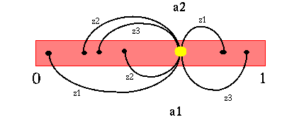
Let us go back to the updating of the belief state discussed earlier. Assume we start with a particular belief state b and we take action a1 and receive observation z1 after taking that action. Then our next belief state is fully determined. In fact, since we are assuming that there are a finite number of actions and a finite number of observations, given a belief state, there are a finite number of possible next belief states. These correspond to each combination of action and observation. The figure below shows this process graphically for a POMDP with two states (s1 and s2), two actions (a1 and a2) and three observations (z1, z2 and z3). The starting belief state is the big yellow dot and the resulting belief states are the smaller black dots. The arcs represent the process of transforming the belief state.
 |
1D belief space for a 2 state POMDP
Note that this shows all possible resulting belief states. Since observations are probabilistic, each resulting belief state has a probability associated with it. More clearly stated: if we take an action and get an observation, then we know with certainty what our next belief state is. However, before we decide to take an action, each resulting belief state has a particular probability associated with it and there are as many possible next belief states as there are observations (for a given action). Note that for a given action, the next belief state probabilities must sum to 1. Also, it is possible that different action-observation combinations could lead to the same belief state, so there may be fewer next belief states than we first mentioned.
It turns out that the process of maintaining the belief state is Markovian; the next belief state depends only on the current belief state (and the current action and observation). In fact, we can convert a discrete POMDP problem into a continuous space CO-MDP problem where the continuous space is the belief space. The transitions of this new continuous space CO-MDP are easily derived from the transition and observation probabilities of the POMDP (remember: no formulas here). What this means is that we are now back to solving a CO-MDP and we can use the value iteration (VI) algorithm. However, we will need to adapt the algorithm some.
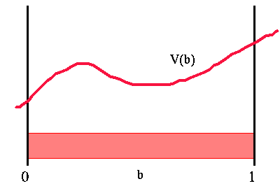
The big problem using value iteration here is the continuous state space. In CO-MDP value iteration we could simply maintain a table with one entry per state. The value of each state is stored in the table and we have a nice finite representation of the value function. Since we now have a continuous space, the value function could be some arbitrary function over belief space. The figure below shows a sample value function over belief space. Here 'b' is a belief space and the value function, 'V(b)', is a function of 'b'. Thus our first problem is how we can easily represent this value function.
 |
Value function over belief space
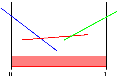
Fortunately, the POMDP formulation imposes some nice restrictions on the form of the solutions to the continuous space CO-MDP that is derived from the POMDP. The key insight is that the finite horizon value function is piecewise linear and convex (PWLC) for every horizon length. This means that for each iteration of value iteration, we only need to find a finite number of linear segments that make up the value function.
The figure below shows a sample value function over belief space for a POMDP. The vertical axis is the value, while the horizontal axis is the belief state. The POMDP value function is the upper surface of a finite number of linear segments. We have colored the segments for a reason to be explained later.
 |
Sample PWLC value function
These linear segments will completely specify the value function (over belief space) that we desire. These amount to nothing more than lines or, more generally, hyper-planes through belief space. We can simply represent each hyper-plane with a vector of numbers, which are the coefficients of the equation of the hyper-plane. The value at any given belief state is found by plugging in the belief state into the hyper-planes equation. If we represent the hyper-plane as a vector (i.e., the equation coefficients) and each belief state as a vector (the probability at each state) then the value of a belief point is simply the dot product of the two vectors. (This is dangerously close to a formula, isn't it?)
We can now represent the value function for each horizon as a set of vectors. To find the value of a belief state, we simply find the vector that has the largest dot product with the belief state.
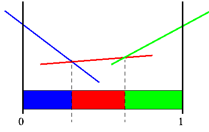
Instead of linear segments over belief space, another way to view the function is that it partitions belief space into a finite number of segments. We will be using both the value function and this partitioning representation to explain the algorithms. Keep in mind that they are more or less interchangeable.
 |
Sample PWLC function and its partition of belief space
Now let's return to the value iteration algorithm. We have a continuous space CO-MDP and we were discussing adapting value iteration to this. The first problem we encountered was how to represent a value function over a continuous space. Since each horizon's value function is PWLC, we solved this problem, by representing the value function as a set of vectors (coefficients of the hyper-planes).
Unfortunately, the continuous space causes us further problems. In each iteration of value iteration in the discrete state space, we would find a state's new value by looping over all the possible next states. However, for continuous state CO-MDPs it is impossible to enumerate all possible states (can you say "uncountably infinite"?).
This is the main obstacle that needs to be overcome and the specific algorithms described later are all different approaches to solve this difficulty. Once we overcome this difficulty, the problem is solved and value iteration works the same here as in the discrete CO-MDP case. The problem now boils down to(可归结为) one stage of value iteration; given a set of vectors representing the value function for horizon 'h', we just need to generate the set of vectors for the value function of horizon 'h+1'
POMDP的更多相关文章
- Variational RL for POMDP
1.Le, Tuan Anh, et al. "Auto-encoding sequential monte carlo." arXiv preprint arXiv:1705.1 ...
- 增强学习(二)----- 马尔可夫决策过程MDP
1. 马尔可夫模型的几类子模型 大家应该还记得马尔科夫链(Markov Chain),了解机器学习的也都知道隐马尔可夫模型(Hidden Markov Model,HMM).它们具有的一个共同性质就是 ...
- 增强学习(三)----- MDP的动态规划解法
上一篇我们已经说到了,增强学习的目的就是求解马尔可夫决策过程(MDP)的最优策略,使其在任意初始状态下,都能获得最大的Vπ值.(本文不考虑非马尔可夫环境和不完全可观测马尔可夫决策过程(POMDP)中的 ...
- 【整理】强化学习与MDP
[入门,来自wiki] 强化学习是机器学习中的一个领域,强调如何基于环境而行动,以取得最大化的预期利益.其灵感来源于心理学中的行为主义理论,即有机体如何在环境给予的奖励或惩罚的刺激下,逐步形成对刺激的 ...
- 论文笔记之:Deep Recurrent Q-Learning for Partially Observable MDPs
Deep Recurrent Q-Learning for Partially Observable MDPs 摘要:DQN 的两个缺陷,分别是:limited memory 和 rely on b ...
- 【cs229-Lecture20】策略搜索
本节内容: 1.POMDP: 2.Policy search算法:reinforced和Pegasus: 马尔科夫决策过程(Partially Observable Markov Decision P ...
- Awesome Reinforcement Learning
Awesome Reinforcement Learning A curated list of resources dedicated to reinforcement learning. We h ...
- 论文笔记之: Recurrent Models of Visual Attention
Recurrent Models of Visual Attention Google DeepMind 模拟人类看东西的方式,我们并非将目光放在整张图像上,尽管有时候会从总体上对目标进行把握,但是也 ...
- 大规模视觉识别挑战赛ILSVRC2015各团队结果和方法 Large Scale Visual Recognition Challenge 2015
Large Scale Visual Recognition Challenge 2015 (ILSVRC2015) Legend: Yellow background = winner in thi ...
随机推荐
- Linux文件(区域)锁函数 -- open()、fcntl()
一.什么是文件锁定 对于锁这个字,大家一定不会陌生,因为我们生活中就存在着大量的锁,它们各个方面发挥着它的作用,现在世界中的锁的功能都可归结为一句话,就是阻止某些人做某些事,例如,门锁就是阻止除了屋主 ...
- 如何对Azure磁盘性能进行测试
Azure的云存储一直是Azure比较自豪的东西,想到AWS的LSA后面有若干个9,搞得大家都以为它的存储最优秀,其实不然,Azure存储到现在没有丢过客户1bit的数据,但是Azure不会去说我们的 ...
- DAY6 使用ping钥匙临时开启SSH:22端口,实现远程安全SSH登录管理就这么简单
设置防火墙策略时,关于SSH:22访问权限,我们常常会设置服务器只接受某个固定IP(如公司IP)访问,但是当我们出差或在家情况需要登录服务器怎么办呢? 常用两种解决方案:1.通过VPN操作登录主机: ...
- canvas案例——画时钟
基本思路,先画一个200半径的圆 ctx.arc(250,250,200,0,2*Math.PI); 然后再画时分刻度,可以先利用translate变化坐标到圆的中心点,然后再通过rotate旋转 / ...
- Memcache 内存分配策略和性能(使用)状态检查
前言: 一直在使用Memcache,但是对其内部的问题,如它内存是怎么样被使用的,使用一段时间后想看看一些状态怎么样?一直都不清楚,查了又忘记,现在整理出该篇文章,方便自己查阅.本文不涉及安装.操作. ...
- SQL Server 2008登录错误:无法连接到(local)解决方法
在一些朋友安装完SQL Server 2008之后大多会遇到连接出错的问题比如:SQL Server 2008登录错误:无法连接到(local)等等相关问题,本文将详细介绍解决方法,需要的朋友可以参考 ...
- 2017 苹果强制https
苹果的ATS(App Transport Security)对服务器硬性3点要求: ① ATS要求TLS1.2或者更高,TLS 是 SSL 新的别称. ② 通讯中的加密套件配置要求支持列出的正向保密. ...
- 使用jquery实现单选框、多选框取消选中状态
function radioReset(){ /*方式一*/ /* var radios = $("input[type='radio']"); for (i=0; i<ra ...
- Android 小笔记
<!-- xml --> android:visibility="gone" 可以隐藏 元素 xmlns:bootstrapbu ...
- Markdown 文档格式编写语法
http://www.cnblogs.com/cxf520/p/6179294.html
