TensorFlow使用记录 (三): Learning Rate Scheduling
file: tensorflow/python/training/learning_rate_decay.py
神经网络中通过超参数 learning rate,来控制每次参数更新的幅度。学习率太小会降低网络优化的速度,增加训练时间;学习率太大则可能导致可能导致参数在局部最优解两侧来回振荡,网络不能收敛。
tensorflow 定义了很多的 学习率衰减方式:
指数衰减 tf.train.exponential_decay()
指数衰减是比较常用的衰减方法,学习率是跟当前的训练轮次指数相关的。
tf.train.exponential_decay(

    learning_rate,     # 初始学习率

    global_step,       # 当前训练轮次

    decay_steps,       # 衰减周期

    decay_rate,        # 衰减率系数

    staircase=False,   # 定义是否是阶梯型衰减,还是连续衰减,默认是 False

    name=None

)

'''

decayed_learning_rate = learning_rate *

                      decay_rate ^ (global_step / decay_steps)

'''
示例代码:
import tensorflow as tf

import matplotlib.pyplot as plt

style1 = []

style2 = []

N = 200

with tf.Session() as sess:

  sess.run(tf.global_variables_initializer())

  for step in range(N):

    # 标准指数型衰减

    learing_rate1 = tf.train.exponential_decay(

      learning_rate=0.5, global_step=step, decay_steps=10, decay_rate=0.9, staircase=False)

    # 阶梯型衰减

    learing_rate2 = tf.train.exponential_decay(

      learning_rate=0.5, global_step=step, decay_steps=10, decay_rate=0.9, staircase=True)

    lr1 = sess.run([learing_rate1])

    lr2 = sess.run([learing_rate2])

    style1.append(lr1)

    style2.append(lr2)

step = range(N)

plt.plot(step, style1, 'g-', linewidth=2, label='exponential_decay')

plt.plot(step, style2, 'r--', linewidth=1, label='exponential_decay_staircase')

plt.title('exponential_decay')

plt.xlabel('step')

plt.ylabel('learing rate')

plt.legend(loc='upper right')

plt.tight_layout()

plt.show()

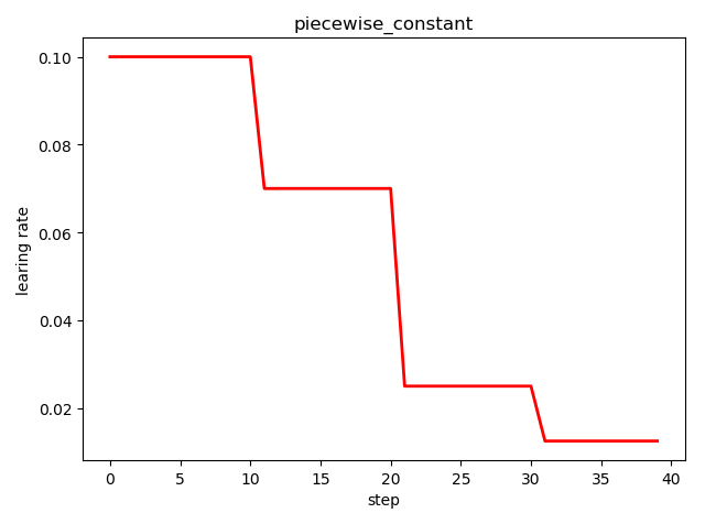
分段常数衰减 tf.train.piecewise_constant()
tf.train.piecewise_constant_decay(

    x,                # 当前训练轮次

    boundaries,       # 学习率应用区间

    values,           # 学习率常数列表

    name=None

)

'''

learning_rate value is `values[0]` when `x <= boundaries[0]`,

    `values[1]` when `x > boundaries[0]` and `x <= boundaries[1]`, ...,

    and values[-1] when `x > boundaries[-1]`.

'''
示例代码:
import tensorflow as tf

import matplotlib.pyplot as plt

boundaries = [10, 20, 30]

learing_rates = [0.1, 0.07, 0.025, 0.0125]

style = []

N = 40

with tf.Session() as sess:

  sess.run(tf.global_variables_initializer())

  for step in range(N):

    learing_rate = tf.train.piecewise_constant(step, boundaries=boundaries, values=learing_rates)

    lr = sess.run([learing_rate])

    style.append(lr)

step = range(N)

plt.plot(step, style, 'r-', linewidth=2)

plt.title('piecewise_constant')

plt.xlabel('step')

plt.ylabel('learing rate')

plt.tight_layout()

plt.show()
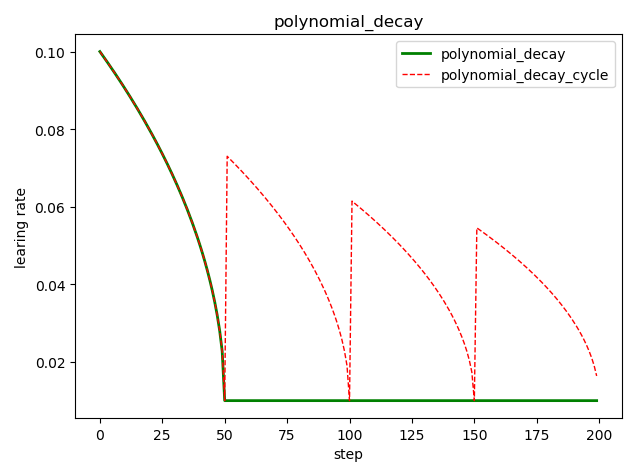
多项式衰减 tf.train.polynomial_decay()
tf.train.polynomial_decay(

    learning_rate,               # 初始学习率

    global_step,                 # 当前训练轮次

    decay_steps,                 # 大衰减周期

    end_learning_rate=0.0001,    # 最小的学习率

    power=1.0,                   # 多项式的幂

    cycle=False,                 # 学习率是否循环

    name=None)

'''

global_step = min(global_step, decay_steps)

decayed_learning_rate = (learning_rate - end_learning_rate) *

                        (1 - global_step / decay_steps) ^ (power) +

                         end_learning_rate

'''
示例代码:
import tensorflow as tf

import matplotlib.pyplot as plt

style1 = []

style2 = []

N = 200

with tf.Session() as sess:

  sess.run(tf.global_variables_initializer())

  for step in range(N):

    # cycle=False

    learing_rate1 = tf.train.polynomial_decay(

      learning_rate=0.1, global_step=step, decay_steps=50,

      end_learning_rate=0.01, power=0.5, cycle=False)

    # cycle=True

    learing_rate2 = tf.train.polynomial_decay(

      learning_rate=0.1, global_step=step, decay_steps=50,

      end_learning_rate=0.01, power=0.5, cycle=True)

    lr1 = sess.run([learing_rate1])

    lr2 = sess.run([learing_rate2])

    style1.append(lr1)

    style2.append(lr2)

steps = range(N)

plt.plot(steps, style1, 'g-', linewidth=2, label='polynomial_decay')

plt.plot(steps, style2, 'r--', linewidth=1, label='polynomial_decay_cycle')

plt.title('polynomial_decay')

plt.xlabel('step')

plt.ylabel('learing rate')

plt.legend(loc='upper right')

plt.tight_layout()

plt.show()
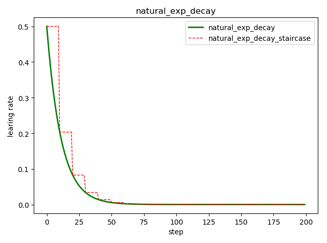
自然指数衰减 tf.train.natural_exp_decay()
tf.train.natural_exp_decay(

    learning_rate,        # 初始学习率

    global_step,          # 当前训练轮次

    decay_steps,          # 衰减周期

    decay_rate,           # 衰减率系数

    staircase=False,      # 定义是否是阶梯型衰减,还是连续衰减,默认是 False

    name=None

)

'''

decayed_learning_rate = learning_rate * exp(-decay_rate * global_step)

'''
示例代码:
import tensorflow as tf

import matplotlib.pyplot as plt

style1 = []

style2 = []

N = 200

with tf.Session() as sess:

  sess.run(tf.global_variables_initializer())

  for step in range(N):

    # 标准指数型衰减

    learing_rate1 = tf.train.natural_exp_decay(

      learning_rate=0.5, global_step=step, decay_steps=10, decay_rate=0.9, staircase=False)

    # 阶梯型衰减

    learing_rate2 = tf.train.natural_exp_decay(

      learning_rate=0.5, global_step=step, decay_steps=10, decay_rate=0.9, staircase=True)

    lr1 = sess.run([learing_rate1])

    lr2 = sess.run([learing_rate2])

    style1.append(lr1)

    style2.append(lr2)

step = range(N)

plt.plot(step, style1, 'g-', linewidth=2, label='natural_exp_decay')

plt.plot(step, style2, 'r--', linewidth=1, label='natural_exp_decay_staircase')

plt.title('natural_exp_decay')

plt.xlabel('step')

plt.ylabel('learing rate')

plt.legend(loc='upper right')

plt.tight_layout()

plt.show()
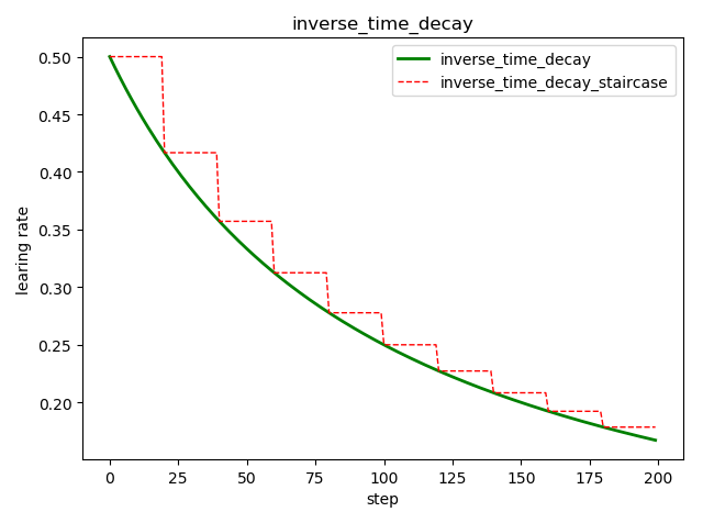
倒数衰减 tf.train.inverse_time_decay()
tf.train.inverse_time_decay(

    learning_rate,     # 初始学习率

    global_step,       # 当前训练轮次

    decay_steps,       # 衰减周期

    decay_rate,        # 衰减率系数

    staircase=False,   # 定义是否是阶梯型衰减,还是连续衰减,默认是 False

    name=None

)

'''

decayed_learning_rate = learning_rate / (1 + decay_rate * global_step / decay_step)

'''
示例代码:
import tensorflow as tf

import matplotlib.pyplot as plt

style1 = []

style2 = []

N = 200

with tf.Session() as sess:

  sess.run(tf.global_variables_initializer())

  for step in range(N):

    # 标准指数型衰减

    learing_rate1 = tf.train.inverse_time_decay(

      learning_rate=0.5, global_step=step, decay_steps=20, decay_rate=0.2, staircase=False)

    # 阶梯型衰减

    learing_rate2 = tf.train.inverse_time_decay(

      learning_rate=0.5, global_step=step, decay_steps=20, decay_rate=0.2, staircase=True)

    lr1 = sess.run([learing_rate1])

    lr2 = sess.run([learing_rate2])

    style1.append(lr1)

    style2.append(lr2)

step = range(N)

plt.plot(step, style1, 'g-', linewidth=2, label='inverse_time_decay')

plt.plot(step, style2, 'r--', linewidth=1, label='inverse_time_decay_staircase')

plt.title('inverse_time_decay')

plt.xlabel('step')

plt.ylabel('learing rate')

plt.legend(loc='upper right')

plt.tight_layout()

plt.show()
余弦衰减 tf.train.cosine_decay()
tf.train.cosine_decay(

    learning_rate,   # 初始学习率

    global_step,     # 当前训练轮次

    decay_steps,     # 衰减周期

    alpha=0.0,       # 最小的学习率

    name=None

)

'''

global_step = min(global_step, decay_steps)

cosine_decay = 0.5 * (1 + cos(pi * global_step / decay_steps))

decayed = (1 - alpha) * cosine_decay + alpha

decayed_learning_rate = learning_rate * decayed

'''
改进的余弦衰减方法还有:
线性余弦衰减,对应函数 tf.train.linear_cosine_decay()
噪声线性余弦衰减,对应函数 tf.train.noisy_linear_cosine_decay()
示例代码:
import tensorflow as tf

import matplotlib.pyplot as plt

style1 = []

style2 = []

style3 = []

N = 200

with tf.Session() as sess:

  sess.run(tf.global_variables_initializer())

  for step in range(N):

    # 余弦衰减

    learing_rate1 = tf.train.cosine_decay(

      learning_rate=0.1, global_step=step, decay_steps=50)

    # 线性余弦衰减

    learing_rate2 = tf.train.linear_cosine_decay(

      learning_rate=0.1, global_step=step, decay_steps=50)

    # 噪声线性余弦衰减

    learing_rate3 = tf.train.noisy_linear_cosine_decay(

      learning_rate=0.1, global_step=step, decay_steps=50,

      initial_variance=0.01, variance_decay=0.1, num_periods=0.2, alpha=0.5, beta=0.2)

    lr1 = sess.run([learing_rate1])

    lr2 = sess.run([learing_rate2])

    lr3 = sess.run([learing_rate3])

    style1.append(lr1)

    style2.append(lr2)

    style3.append(lr3)

step = range(N)

plt.plot(step, style1, 'g-', linewidth=2, label='cosine_decay')

plt.plot(step, style2, 'r--', linewidth=1, label='linear_cosine_decay')

plt.plot(step, style3, 'b--', linewidth=1, label='linear_cosine_decay')

plt.title('cosine_decay')

plt.xlabel('step')

plt.ylabel('learing rate')

plt.legend(loc='upper right')

plt.tight_layout()

plt.show()

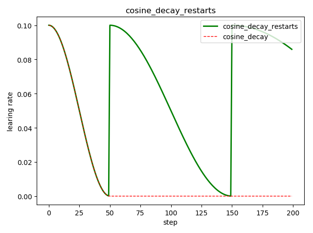
循环余弦衰减 tf.train.cosine_decay_restarts()
这是在 fast.ai 中强推的衰减方式
tf.train.cosine_decay_restarts(

    learning_rate,      # 初始学习率

    global_step,        # 当前训练轮次

    first_decay_steps,  # 首次衰减周期

    t_mul=2.0,          # 随后每次衰减周期倍数

    m_mul=1.0,          # 随后每次初始学习率倍数

    alpha=0.0,          # 最小的学习率=alpha*learning_rate

    name=None

)

'''

See [Loshchilov & Hutter, ICLR2016], SGDR: Stochastic Gradient Descent

with Warm Restarts. https://arxiv.org/abs/1608.03983

The learning rate multiplier first decays

from 1 to `alpha` for `first_decay_steps` steps. Then, a warm

restart is performed. Each new warm restart runs for `t_mul` times more steps

and with `m_mul` times smaller initial learning rate.

'''
示例代码:
import tensorflow as tf

import matplotlib.pyplot as plt

style1 = []

style2 = []

N = 200

with tf.Session() as sess:

  sess.run(tf.global_variables_initializer())

  for step in range(N):

    # 循环余弦衰减

    learing_rate1 = tf.train.cosine_decay_restarts(

      learning_rate=0.1, global_step=step, first_decay_steps=50,

      )

    # 余弦衰减

    learing_rate2 = tf.train.cosine_decay(

      learning_rate=0.1, global_step=step, decay_steps=50)

    lr1 = sess.run([learing_rate1])

    lr2 = sess.run([learing_rate2])

    style1.append(lr1)

    style2.append(lr2)

step = range(N)

plt.plot(step, style1, 'g-', linewidth=2, label='cosine_decay_restarts')

plt.plot(step, style2, 'r--', linewidth=1, label='cosine_decay')

plt.title('cosine_decay_restarts')

plt.xlabel('step')

plt.ylabel('learing rate')

plt.legend(loc='upper right')

plt.tight_layout()

plt.show()
调用例子
import tensorflow as tf

def Swish(features):

    return features*tf.nn.sigmoid(features)

# 1. create data

from tensorflow.examples.tutorials.mnist import input_data

mnist = input_data.read_data_sets('../MNIST_data', one_hot=True)

X = tf.placeholder(tf.float32, shape=(None, 784), name='X')

y = tf.placeholder(tf.int32, shape=(None), name='y')

is_training = tf.placeholder(tf.bool, None, name='is_training')

# 2. define network

he_init = tf.contrib.layers.variance_scaling_initializer()

with tf.name_scope('dnn'):

    hidden1 = tf.layers.dense(X, 300, kernel_initializer=he_init, name='hidden1')

    hidden1 = tf.layers.batch_normalization(hidden1, momentum=0.9)

    hidden1 = tf.nn.relu(hidden1)

    hidden2 = tf.layers.dense(hidden1, 100, kernel_initializer=he_init, name='hidden2')

    hidden2 = tf.layers.batch_normalization(hidden2, training=is_training, momentum=0.9)

    hidden2 = tf.nn.relu(hidden2)

    logits = tf.layers.dense(hidden2, 10, kernel_initializer=he_init, name='output')

    # prob = tf.layers.dense(hidden2, 10, tf.nn.softmax, name='prob')

# 3. define loss

with tf.name_scope('loss'):

    # tf.losses.sparse_softmax_cross_entropy() label is not one_hot and dtype is int*

    # xentropy = tf.losses.sparse_softmax_cross_entropy(labels=tf.argmax(y, axis=1), logits=logits)

    # tf.nn.sparse_softmax_cross_entropy_with_logits() label is not one_hot and dtype is int*

    # xentropy = tf.nn.sparse_softmax_cross_entropy_with_logits(labels=tf.argmax(y, axis=1), logits=logits)

    # loss = tf.reduce_mean(xentropy)

    loss = tf.losses.softmax_cross_entropy(onehot_labels=y, logits=logits) # label is one_hot

# 4. define optimizer

learning_rate_init = 0.01

global_step = tf.Variable(0, trainable=False)

with tf.name_scope('train'):

    learning_rate = tf.train.polynomial_decay(  # 多项式衰减

        learning_rate=learning_rate_init,  # 初始学习率

        global_step=global_step,  # 当前迭代次数

        decay_steps=22000,  # 在迭代到该次数实际,学习率衰减为 learning_rate * dacay_rate

        end_learning_rate=learning_rate_init / 10,  # 最小的学习率

        power=0.9,

        cycle=False

    )

    update_ops = tf.get_collection(tf.GraphKeys.UPDATE_OPS)  # for batch normalization

    with tf.control_dependencies(update_ops):

        optimizer_op = tf.train.GradientDescentOptimizer(

            learning_rate=learning_rate).minimize(

            loss=loss,

            var_list=tf.trainable_variables(),

            global_step=global_step # 不指定的话学习率不更新

        )

        # ================= clip gradient

        # threshold = 1.0

        # optimizer = tf.train.GradientDescentOptimizer(learning_rate)

        # grads_and_vars = optimizer.compute_gradients(loss)

        # capped_gvs = [(tf.clip_by_value(grad, -threshold, threshold), var)

        #               for grad, var in grads_and_vars]

        # optimizer_op = optimizer.apply_gradients(capped_gvs)

        # =================

with tf.name_scope('eval'):

    correct = tf.nn.in_top_k(logits, tf.argmax(y, axis=1), 1) # 目标是否在前K个预测中, label's dtype is int*

    accuracy = tf.reduce_mean(tf.cast(correct, tf.float32))

# 5. initialize

init_op = tf.group(tf.global_variables_initializer(), tf.local_variables_initializer())

saver = tf.train.Saver()

# =================

print([v.name for v in tf.trainable_variables()])

print([v.name for v in tf.global_variables()])

# =================

# 6. train & test

n_epochs = 20

n_batches = 50

batch_size = 50

with tf.Session() as sess:

    sess.run(init_op)

    # saver.restore(sess, './my_model_final.ckpt')

    for epoch in range(n_epochs):

        for iteration in range(mnist.train.num_examples // batch_size):

            X_batch, y_batch = mnist.train.next_batch(batch_size)

            sess.run([optimizer_op, learning_rate], feed_dict={X: X_batch, y: y_batch, is_training:True})

            # ================= check gradient

            # for grad, var in grads_and_vars:

            #     grad = grad.eval(feed_dict={X: X_batch, y: y_batch, is_training:True})

            #     var = var.eval()

            # =================

        learning_rate_cur = learning_rate.eval()

        acc_train = accuracy.eval(feed_dict={X: X_batch, y: y_batch, is_training:False}) # 最后一个 batch 的 accuracy

        acc_test = accuracy.eval(feed_dict={X: mnist.test.images, y: mnist.test.labels, is_training:False})

        loss_test = loss.eval(feed_dict={X: mnist.test.images, y: mnist.test.labels, is_training:False})

        print(epoch, "Current learning rate:", learning_rate_cur, "Train accuracy:", acc_train, "Test accuracy:", acc_test, "Test loss:", loss_test)

    save_path = saver.save(sess, "./my_model_final.ckpt")

with tf.Session() as sess:

    sess.run(init_op)

    saver.restore(sess, "./my_model_final.ckpt")

    acc_test = accuracy.eval(feed_dict={X: mnist.test.images, y: mnist.test.labels, is_training:False})

    loss_test = loss.eval(feed_dict={X: mnist.test.images, y: mnist.test.labels, is_training:False})

    print("Test accuracy:", acc_test, ", Test loss:", loss_test)
Since AdaGrad, RMSProp, and Adam optimization automatically reduce the learning rate during training, it is not necessary to add an extra learning schedule. For other optimization algorithms, using exponential decay or performance scheduling can considerably speed up convergence.
TensorFlow使用记录 (三): Learning Rate Scheduling的更多相关文章
- 5、Tensorflow基础(三)神经元函数及优化方法
1.激活函数 激活函数(activation function)运行时激活神经网络中某一部分神经元,将激活信息向后传入下一层的神经网络.神经网络之所以能解决非线性问题(如语音.图像识别),本质上就是激 ...
- Deep Learning 32: 自己写的keras的一个callbacks函数,解决keras中不能在每个epoch实时显示学习速率learning rate的问题
一.问题: keras中不能在每个epoch实时显示学习速率learning rate,从而方便调试,实际上也是为了调试解决这个问题:Deep Learning 31: 不同版本的keras,对同样的 ...
- TensorFlow使用记录 (九): 模型保存与恢复
模型文件 tensorflow 训练保存的模型注意包含两个部分:网络结构和参数值. .meta .meta 文件以 “protocol buffer”格式保存了整个模型的结构图,模型上定义的操作等信息 ...
- TensorFlow使用记录 (六): 优化器
0. tf.train.Optimizer tensorflow 里提供了丰富的优化器,这些优化器都继承与 Optimizer 这个类.class Optimizer 有一些方法,这里简单介绍下: 0 ...
- tensorflow笔记(三)之 tensorboard的使用
tensorflow笔记(三)之 tensorboard的使用 版权声明:本文为博主原创文章,转载请指明转载地址 http://www.cnblogs.com/fydeblog/p/7429344.h ...
- mxnet设置动态学习率(learning rate)
https://blog.csdn.net/xiaotao_1/article/details/78874336 如果learning rate很大,算法会在局部最优点附近来回跳动,不会收敛: 如果l ...
- TensorFlow使用记录 (八): 梯度修剪 和 Max-Norm Regularization
梯度修剪 梯度修剪主要避免训练梯度爆炸的问题,一般来说使用了 Batch Normalization 就不必要使用梯度修剪了,但还是有必要理解下实现的 In TensorFlow, the optim ...
- TensorFlow实战第三课(可视化、加速神经网络训练)
matplotlib可视化 构件图形 用散点图描述真实数据之间的关系(plt.ion()用于连续显示) # plot the real data fig = plt.figure() ax = fig ...
- Dynamic learning rate in training - 培训中的动态学习率
I'm using keras 2.1.* and want to change the learning rate during training. I know about the schedul ...
随机推荐
- SQL SERVER 字符串函数 STUFF()
说明: STUFF 函数将字符串插入到另一个字符串中. 它从第一个字符串的开始位置删除指定长度的字符:然后将第二个字符串插入到第一个字符串的开始位置. 语法: STUFF ( character_ex ...
- ABC143F Distinct Numbers
这道题非常好.其思想类似于 $O(n \log n)$ 求最长上升子序列的算法. hint:考虑固定操作次数 $o$,$k$ 最大可取到多少? int n; scan(n); vi a(n); sca ...
- Java白皮书学习笔记+Head First Java--用于自我复习 基础知识篇
本笔记是摘与Hava白皮书上面的内容,用来给自己做提醒的,因此大概并不适合Java的学习者作为笔记参考使用. 以我的水平现在还看不懂这个... 一.基础知识篇 1.常量 final关键字指示常量,只能 ...
- The Party and Sweets CodeForces - 1159C (拓排)
优化连边然后拓排. #include <iostream> #include <sstream> #include <algorithm> #include < ...
- java构造方法的注意事项总结
构造方法细节总结~~~~~ 1:首先要了解为什么需要构造方法,,,类中有太多的属性,每次给属性赋值时非常麻烦:编码量大,无法重用给属性赋值的代码.. 2:什么是构造方法呢? 构造方法负责初始化类中的实 ...
- 100、神器的 routing mesh (Swarm07)
参考https://www.cnblogs.com/CloudMan6/p/7930321.html 上一节我们提到了 swarm 的 routing mesh .当外部访问任意节点的8080端口 ...
- vue路由守卫触发顺序
不同组件之间的路由跳转流程图 导航被触发(A–>B) 调用A组件内路由守卫beforeRouteLeave(to,from,next) 调用全局路由前置守卫router.beforeEach(t ...
- python之multiprocessing多进程
multiprocessing 充分利用cpu多核一般情况下cpu密集使用进程池,IO密集使用线程池.python下想要充分利用多核CPU,就用多进程. Process 类Process 类用来描述一 ...
- Java注解的继承
注解继承的说明 1.首先要想Annotation能被继承,需要在注解定义的时候加上@Inherited,并且如果要被反射应用的话,就需要还有个事@Retention(RetentionPolicy.R ...
- lftp连接异常情况分析过程
[问题现象]:通过rpm安装好lftp后,执行lftp huangmr:huangmr@192.168.107.132无法连接(lftp huangmr@192.168.107.132:~> l ...