【PyTorch】常用的神经网络层汇总（持续补充更新）

1. Convolution Layers

1.1 nn.Conv2d

（1）原型

torch.nn.Conv2d(in_channels, out_channels, kernel_size, stride=1, padding=0, dilation=1, groups=1, bias=True,

                padding_mode='zeros', device=None, dtype=None)

　　在由多个输入平面组成的输入信号上应用2D卷积，简言之就是在多通道输入图像上进行卷积操作。

（2）参数

in_channels (int) — 输入图像的通道数

out_channels (int) — 输出图像（张量表示）的通道数

kernel_size (int or tuple) — 卷积核大小。n*n型的写成 kernel_size = 5 即可，n*m型的则需要写成 kernel_size = (n, m)

stride (int or tuple, 可选择) — 卷积步长，即卷积核在图像上每次平移的间隔。默认：1

padding (int, tuple or str, 可选择) — 边缘填充，图像上下左右四边填充为 0 的行数和列数。默认：0

padding_mode (string, 可选择) — padding的模式：'zeros'，’reflect'，'replicata' 或 'circular'。默认：'zeros'

dilation (int or tuple, 可选择) — 内核元素的间隔，该参数决定了是否采用空洞卷积。默认：1（不采用）

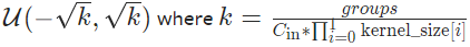
groups (int, 可选择) — 输入通道到输出通道之间块状连接的数量。默认：1

bias (bool, 可选择) — 是否增加一个可学习的偏置项到输出。默认：True

（3）属性

~Linear.weight (torch.Tensor) — 形状为 (out_channels, in_channels / group, kernel_size[0], kernel_size[1]) 的模型的可学习的偏置项

初始化为：

~Linear.bias — 形状为 (out_channels) 的模型的可学习的偏置项

如果bias为True，初始化为：

（4）用法示例

import torch

import torch.nn as nn

m = nn.Conv2d(16, 33, (3, 5), stride=(2, 1), padding=(4, 2), dilation=(3, 1))

print(m)

# (N, C, H, W)

inputImage = torch.randn(20, 16, 50, 100)

output = m(inputImage)

print(output.shape)

结果：

2. Pooling Layers

2.1 nn.MaxPool2d

（1）原型

torch.nn.MaxPool2d(kernel_size, stride=None, padding=0, dilation=1, return_indices=False, ceil_mode=False)

在由多个输入平面组成的输入信号上应用 2D 最大池化。

注：当 ceil_mode=True 时，如果滑动窗口从左侧填充或输入中开始，则允许它们越界。在右侧填充区域开始的滑动窗口将被忽略。

（2）参数

kernel_size — 表示做最大池化的窗口大小，可以是单个值，也可以是tuple元组
stride — 卷积步长，即卷积核在图像上每次平移的间隔。默认：kernel_size

padding — 图像上下左右四边填充为 0 的行数和列数。默认：0
dilation — 内核元素的间隔，该参数决定了是否采用空洞卷积。默认：1（不采用）
return_indices (bool) — 是否返回输出的最大索引。默认：False
ceil_mode (bool) — 使用向上取整（ceil）或向下取整（floor）的方式计算得到输出形状。默认：False（floor，向下取整）

（3）用法示例

# pool of square window of size=3, stride=2

m = nn.MaxPool2d(3, stride=2)

# pool of non-square window

m = nn.MaxPool2d((3, 2), stride=(2, 1))

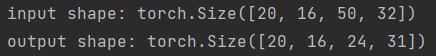
input = torch.randn(20, 16, 50, 32)

output = m(input)

print(f'input shape: {input.shape}', f'output shape: {output.shape}', sep='\n')

结果：

2.2 nn.AvgPool2d

（1）原型

torch.nn.AvgPool2d(kernel_size, stride=None, padding=0, ceil_mode=False, count_include_pad=True, divisor_override=None)

在由多个输入平面组成的输入信号上应用 2D 平均池化。

注：当 ceil_mode=True 时，如果滑动窗口从左侧填充或输入中开始，则允许它们越界。在右侧填充区域开始的滑动窗口将被忽略。

（2）参数

kernel_size — 表示做最大池化的窗口大小，可以是单个值，也可以是tuple元组
stride — 卷积步长，即卷积核在图像上每次平移的间隔。默认：kernel_size
padding — 图像上下左右四边填充为 0 的行数和列数。默认：0
ceil_mode — 使用向上取整（ceil）或向下取整（floor）的方式计算得到输出形状。默认：False（floor，向下取整）
count_include_pad — 是否在平均计算中包含零填充。默认：True
divisor_override — 如果指定，它将用作除数，否则将使用池化区域的大小

（3）用法示例

# pool of square window of size=3, stride=2

m = nn.AvgPool2d(3, stride=2)

# pool of non-square window

m = nn.AvgPool2d((3, 2), stride=(2, 1))

input = torch.randn(20, 16, 50, 32)

output = m(input)

print(f'\ninput shape: {input.shape}', f'output shape: {output.shape}', sep='\n')

2.3 AdaptiveMaxPool2d

（1）原型

torch.nn.AdaptiveMaxPool2d(output_size, return_indices=False)

在由多个输入平面组成的输入信号上应用 2D 自适应最大池化。

对于任何输入大小，输出大小为 H_out * W_out，输出特征的数量等于输入平面的数量。

（2）参数

output_size — 目标输出为形如 H_out * W_out 的图像。可能是一个数组 (H_out, W_out) 或者方形图像 H_out * H_out的单项 H_out 。H_out 和 W_out可以是 int，也可以是 None，这意味着大小将与输入的大小相同
return_indices — 是否返回输出的最大索引。默认：False

（3）用法

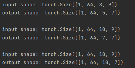
# target output size of 5x7

m = nn.AdaptiveMaxPool2d((5, 7))

input = torch.randn(1, 64, 8, 9)

output = m(input)

print(f'input shape: {input.shape}', f'output shape: {output.shape}', sep='\n')

# target output size of 7x7 (square)

m = nn.AdaptiveMaxPool2d(7)

input = torch.randn(1, 64, 10, 9)

output = m(input)

print(f'\ninput shape: {input.shape}', f'output shape: {output.shape}', sep='\n')

# target output size of 10x7

m = nn.AdaptiveMaxPool2d((None, 7))

input = torch.randn(1, 64, 10, 9)

output = m(input)

print(f'\ninput shape: {input.shape}', f'output shape: {output.shape}', sep='\n')

结果：

2.4 AdaptiveAvgPool2d

（1）原型

torch.nn.AdaptiveAvgPool2d(output_size)

在由多个输入平面组成的输入信号上应用 2D 自适应平均池化。

对于任何输入大小，输出大小为 H x W。输出特征的数量等于输入平面的数量。

（2）参数

output_size – 目标输出为形如 H * W 的图像。可能是一个数组 (H, W) 或者方形图像 H * H的单项 H 。H 和 W可以是 int，也可以是 None，这意味着大小将与输入的大小相同

（3）用法

# target output size of 5x7

m = nn.AdaptiveAvgPool2d((5, 7))

input = torch.randn(1, 64, 8, 9)

output = m(input)

print(f'input shape: {input.shape}', f'output shape: {output.shape}', sep='\n')

# target output size of 7x7 (square)

m = nn.AdaptiveAvgPool2d(7)

input = torch.randn(1, 64, 10, 9)

output = m(input)

print(f'\ninput shape: {input.shape}', f'output shape: {output.shape}', sep='\n')

# target output size of 10x7

m = nn.AdaptiveAvgPool2d((None, 7))

input = torch.randn(1, 64, 10, 9)

output = m(input)

print(f'\ninput shape: {input.shape}', f'output shape: {output.shape}', sep='\n')

3. Non-linear Activations (weighted sum, nonlinearity)

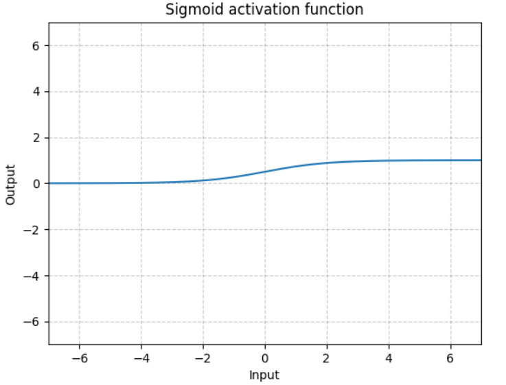
3.1 nn.Sigmoid

（1）原型

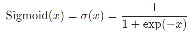
torch.nn.Sigmoid()

（2）Sigmoid函数表达式及图像

逐元素执行：

（3）用法示例

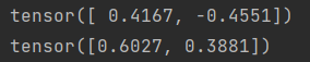
m = nn.Sigmoid()

input = torch.randn(2)

print(input)

output = m(input)

print(output)

结果：

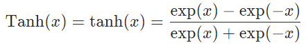
3.2 nn.Tanh

（1）原型

torch.nn.Tanh()

（2）Tanh函数表达式及图像

逐元素执行：

（3）用法示例

m = nn.Tanh()

input = torch.randn(2)

print(input)

output = m(input)

print(output)

结果：

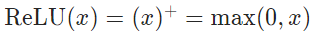
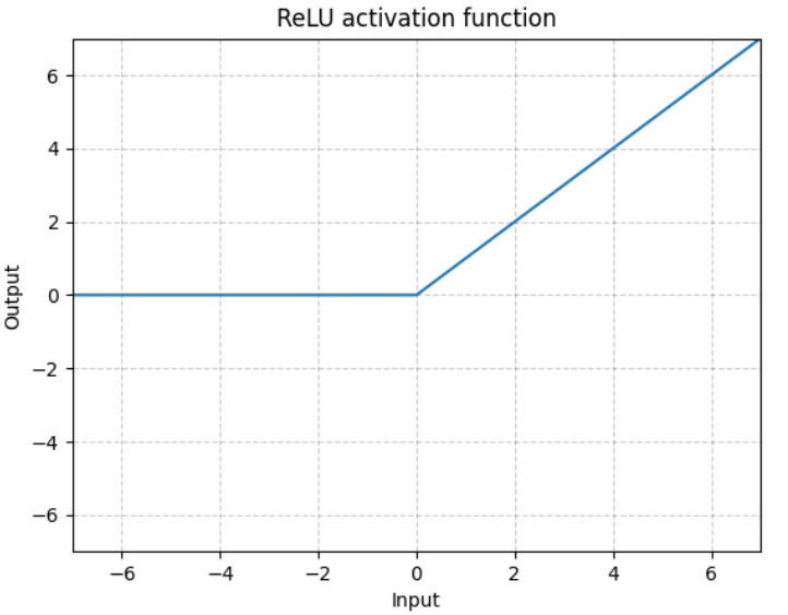
3.3 nn.ReLU

（1）原型

torch.nn.ReLU(inplace=False)

（2）ReLU函数表达式及图像

逐元素执行：

（3）参数

inplace — 选择是否就地执行操作，即是否对Input本身执行该操作。若为True，则对Input执行ReLU的同时也会改变（或刷新）Input的值，使得Input=Output；若为False，则不会改变Input的值。默认：False

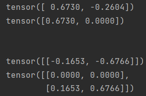
（4）用法示例

m = nn.ReLU()

input = torch.randn(2)

output = m(input)

# An implementation of CReLU - https://arxiv.org/abs/1603.05201

m = nn.ReLU()

input = torch.randn(2).unsqueeze(0)

output = torch.cat((m(input),m(-input)))

结果：

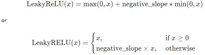
3.4 nn.LeakyReLU

（1）定义

torch.nn.LeakyReLU(negative_slope=0.01, inplace=False)

（2）LeakyReLU函数表达式和图像

逐元素执行：

（3）参数

negative_slope — Input的负数部分的斜率。默认：1e-2
inplace — 选择是否就地执行操作，即是否对Input本身执行该操作。若为True，则对Input执行ReLU的同时也会改变（或刷新）Input的值，使得Input=Output；若为False，则不会改变Input的值。默认：False

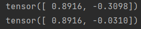
（4）用法示例

m = nn.LeakyReLU(0.1)

input = torch.randn(2)

print(input)

output = m(input)

print(output)

结果：

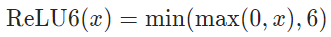
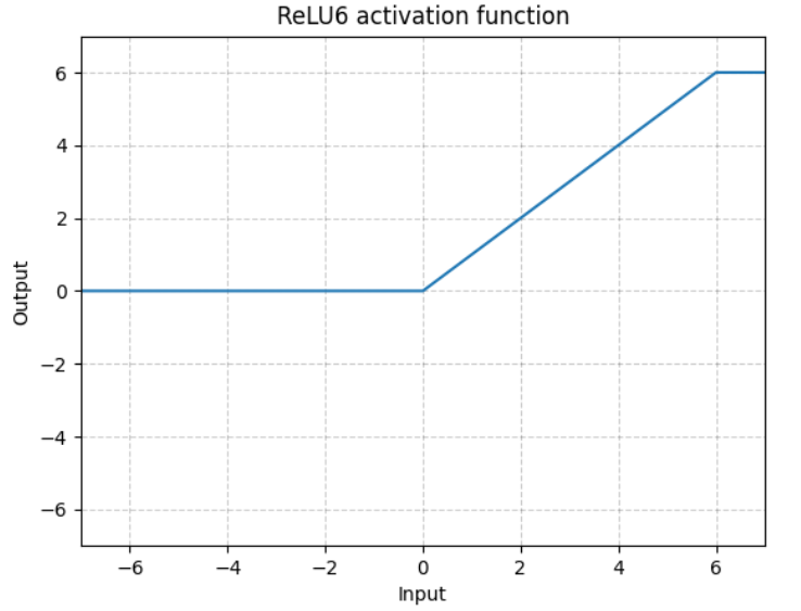
3.5 nn.ReLU6

（1）原型

torch.nn.ReLU6(inplace=False)

（2）ReLU6函数表达式及图像

逐元素执行：

（3）参数

inplace — 选择是否就地执行操作，即是否对Input本身执行该操作。若为True，则对Input执行ReLU的同时也会改变（或刷新）Input的值，使得Input=Output；若为False，则不会改变Input的值。默认：False

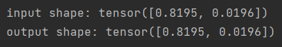
（4）用法示例

m = nn.ReLU6()

input = torch.randn(2)

output = m(input)

print(f'input shape: {input}', f'output shape: {output}', sep='\n')

结果：

3.6 nn.GeLU

（1）原型

torch.nn.GELU

（2）GELU函数表达式及图像

逐元素执行：

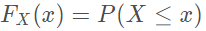
是高斯分布的累积分布函数（概率密度函数的积分），表示如下：

（3）用法示例

# GeLU

m = nn.GELU()

input = torch.randn(2)

output = m(input)

print('input: ', input, 'output: ', output, sep='\n')

结果：

3.7 nn.SeLU

（1）原型

torch.nn.SELU(inplace=False)

注：当使用 kaiming_normal 或 kaiming_normal_ 进行初始化时，应使用 nonlinearity='linear' 而不是 nonlinearity='selu'，以获得自归一化神经网络。

更多细节详见 Self-Normalizing Neural Networks 一文。

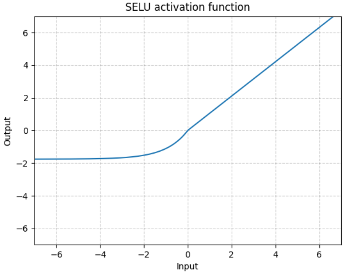
（2）SELU函数表达式及图像

逐元素执行：

式中：α=1.6732632423543772848170429916717，scale=1.0507009873554804934193349852946

（3）参数

inplace（bool, 可选择）— 选择是否就地执行操作，即是否对Input本身执行该操作。若为True，则对Input执行ReLU的同时也会改变（或刷新）Input的值，使得Input=Output；若为False，则不会改变Input的值。默认：False

（4）用法示例

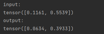
# SeLU

m = nn.SELU()

input = torch.randn(2)

output = m(input)

print('input: ', input, 'output: ', output, sep='\n')

结果：

4. Non-linear Activations (other)

4.1 nn.Softmax

（1）原型

torch.nn.Softmax(dim=None)

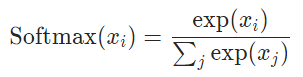
将 Softmax 函数应用于 n 维的输入张量，改变他们的大小，使得 n 维输出张量的元素位于 [0, 1] 范围内，并且总和为0。

当输入张量是稀疏张量时，未指定的值将被视为 -inf。

需要注意的是，该模块不直接与 NLLLoss 一起使用，它期望在 Softmax 和自身之间计算 Log。改用 LogSoftmax（它更快并且具有更好的数值属性）

（2）Softmax函数表达式

（3）参数

dim (int) — 计算 Softmax 的维度（因此沿 dim 的每个切片总和为 1）。

（4）用法示例

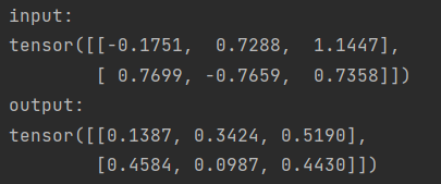
# Softmax

m = nn.Softmax(dim=1)

input = torch.randn(2, 3)

output = m(input)

print('input: ', input, 'output: ', output, sep='\n')

结果：

5 . Normalization Layers

5.1 nn.BatchNorm2d

（1）原型

torch.nn.BatchNorm2d(num_features, eps=1e-05, momentum=0.1, affine=True,

                     track_running_stats=True, device=None, dtype=None)

对4D输入应用批量归一化（具有附加通道尺寸的小批量的2D输入）。详述可参考论文 Batch Normalization: Accelerating Deep Network Training by Reducing Internal Covariate Shift .

（2）参数

num_features — 指特征数。一般情况下输入的数据格式为（batch_size，num_features，height，width）其中的C为特征数，也称channel数
eps — 为了分数值稳定而添加到分母的值。默认：1e-5
momentum — 用于运行过程中均值和方差的估计参数。可以将累积移动平均线（即简单平均线）设置为 None 。默认：0.1
affine — 此模块是否具有可学习的仿射参数。默认：True
track_running_stats — 一个布尔值，当设置为True时，此模块跟踪运行平均值和方差；设置为False时，此模块不跟踪此类统计信息，并将统计信息缓冲区running_mean和running_var初始化为None。当这些缓冲区为None时，此模块将始终使用批处理统计信息。在训练和评估模式下都可以。默认：True

（3）用法示例

# With Learnable Parameters

m = nn.BatchNorm2d(100)

# Without Learnable Parameters

m = nn.BatchNorm2d(100, affine=False)

input = torch.randn(20, 100, 35, 45)

output = m(input)

6. Linear Layers

6.1 nn.Linear

（1）原型

torch.nn.Linear(in_features, out_features, bias=True, device=None, dtype=None)

对输入数据进行线性变换：

（2）参数

in_features — 每个输入样本的尺寸
out_features — 每个输出样本的尺寸
bias — 该层是否会学习一个额外的偏置项。默认：True
device — 代表将分配到设备的对象（'cpu' 或 'cuda'，cuda需设置设备编号，比如 'cuda:0'、'cuda:1' 等）

dtype — 代表数据类型

（3）属性

~Linear.weight (torch.Tensor) — 形状为（out_features, in_features）的模型的可学习的偏置项

初始化为：

~Linear.bias — 形状为out_features的模型的可学习的偏置项

如果bias为True，初始化为：

（4）用法示例

# Linear

m = nn.Linear(20, 30)

input = torch.randn(128, 20)

output = m(input)

print(f'output size: {output.size()}', f'weight size: {m.weight.size()}', f'bias size: {m.bias.size()}', sep='\n')

结果：

7. Dropout Layers

7.1 nn.Dropout

（1）原型

torch.nn.Dropout(p=0.5, inplace=False)

在训练期间，使用来自伯努利分布的样本以概率 p 将输入张量的一些元素随机归零。每个通道将在每次前向调用时独立归零。

Dropout是一种用于正则化和防止神经元间互适应的有效技术，详细介绍可参考 Improving neural networks by preventing co-adaptation of feature detectors 一文。此外，输出在训练期间按 1/(1-p) 倍缩放。这意味着在评估期间，模块只计算一个恒等函数。

输入可以是任意形状的张量，输出形状与输入保持一致。

（2）参数

p — 元素归零的概率。默认：0.5
inplace — 选择是否就地执行操作，即是否对Input本身执行该操作。若为True，则对Input执行ReLU的同时也会改变（或刷新）Input的值，使得Input=Output；若为False，则不会改变Input的值。默认：False

（3）用法示例

# Dropout

m = nn.Dropout(p=0.2)

input = torch.randn(4, 6)

output = m(input)

print('input:', input, 'output:', output, sep='\n')

结果：

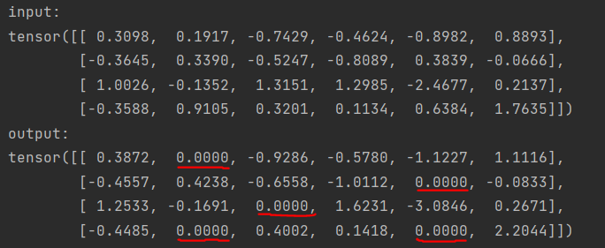
问：除了以 p=0.2 的概率随机归零的一些元素以外，其他元素的值为什么也变化了？

答：所有的元素都会在训练期间按 1/(1-p) 倍缩放。

7.2 nn.Dropout2d

（1）原型

torch.nn.Dropout2d(p=0.5, inplace=False)

不同于前一节的Dropout，Dropout2d是将整个通道随机归零（一个通道通常代表一个2D特征图，比如：在批量输入中，第 i 个样本的第 j 个通道是一个2D的张量 input[i, j]），使用来自伯努利分布的样本，每个通道将在每次前向调用中使用来自伯努利分布的样本以概率 p 独立清零。

如论文 Efficient Object Localization Using Convolutional Networks 中所述，如果特征图中的相邻像素是强相关的（通常在早期卷积层中就是这种情况），那么 dropout 不会规范激活，否则只会导致有效的学习率降低。在这种情况下，nn.Dropout2d() 将有助于促进特征图之间的独立性，应改为使用。

输入可以是 (N, C, H, W) 或 (C, H, W) ，输出和输入形状一致，也是(N, C, H, W) 或 (C, H, W) 。

（2）参数

p — 元素归零的概率。默认：0.5
inplace — 选择是否就地执行操作，即是否对Input本身执行该操作。若为True，则对Input执行ReLU的同时也会改变（或刷新）Input的值，使得Input=Output；若为False，则不会改变Input的值。默认：False

（3）用法示例

# Dropout

m = nn.Dropout(p=0.2)

input = torch.randn(4, 6)

output = m(input)

print('input:', input, 'output:', output, sep='\n')

结果：

8. Loss Functions

8.1 nn.L1Loss

（1）原型

torch.nn.L1Loss(size_average=None, reduce=None, reduction='mean')

计算输入 x 和目标 y 之间的平均绝对误差（MAE）。x可以是任意维度的张量；y形状和x保持一致。

（2）公式

（3）参数

size_average (bool, 可选参数) — 已弃用（参考reduction参数）。默认情况下，损失是批次中每个损失元素的平均值。请注意，对于某些损失，每个样本有多个元素。如果字段 size_average 设置为 False，则将每个 minibatch 的损失相加。当 reduce 为 False 时忽略。默认：True
reduce (bool, 可选参数) — 已弃用（参考reduction参数）。默认情况下，损失会根据 size_average 对每个小批量的观测值进行平均或求和。当 reduce 为 False 时，返回每个批次元素的损失并忽略 size_average。默认：True
reduction (string, 可选参数) — 指定要用于输出的reduction取值：none，mean，sum。none：不使用reduction；mean：输出的总和将除以输出中的元素数；sum：输出将被求和。注意：size_average 和 reduce 正在被弃用，同时，指定这两个参数中的任何一个都将覆盖 reduction。默认：mean

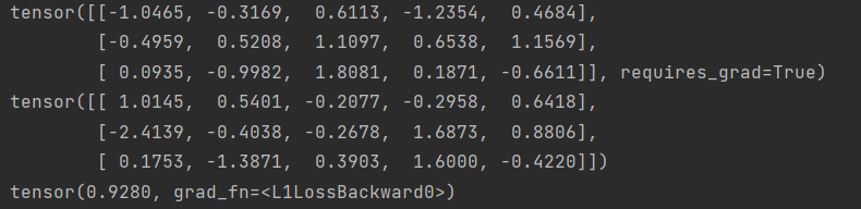
（4）用法

# L1Loss

loss = nn.L1Loss()

input = torch.randn(3, 5, requires_grad=True)

target = torch.randn(3, 5)

output = loss(input, target)

output.backward()

print(input, target, output, sep='\n')

结果：

8.2 nn.MSELoss（L2Loss）

（1）原型

torch.nn.MSELoss(size_average=None, reduce=None, reduction='mean')

计算输入 x 和目标 y 中的每个元素之间的均方误差（平方 L2 范数）

（2）公式

（3）参数

size_average (bool, 可选参数) — 已弃用（参考reduction参数）。默认情况下，损失是批次中每个损失元素的平均值。请注意，对于某些损失，每个样本有多个元素。如果字段 size_average 设置为 False，则将每个 minibatch 的损失相加。当 reduce 为 False 时忽略。默认：True
reduce (bool, 可选参数) — 已弃用（参考reduction参数）。默认情况下，损失会根据 size_average 对每个小批量的观测值进行平均或求和。当 reduce 为 False 时，返回每个批次元素的损失并忽略 size_average。默认：True
reduction (string, 可选参数) — 指定要用于输出的reduction取值：none，mean，sum。none：不使用 reduction；mean：输出的总和将除以输出中的元素数；sum：输出将被求和。注意：size_average 和 reduce 正在被弃用，同时，指定这两个参数中的任何一个都将覆盖 reduction。默认：mean

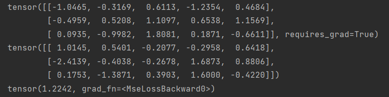
（4）用法

# MSELoss(L2Loss)

loss = nn.MSELoss()

input = torch.randn(3, 5, requires_grad=True)

target = torch.randn(3, 5)

output = loss(input, target)

output.backward()

print(input, target, output, sep='\n')

结果：

8.3 nn.CrossEntropyLoss

（1）原型

torch.nn.CrossEntropyLoss(weight=None, size_average=None, ignore_index=- 100, reduce=None, reduction='mean', label_smoothing=0.0)

计算输入 x 和目标 y 之间的交叉熵损失

（2）公式

（3）参数

weight (Tensor, 可选参数) – 手动重新调整每个类别的权重。如果给定，则必须是大小为 C 的张量
size_average (bool, 可选参数) – 已弃用（参考reduction参数）。默认情况下，损失是批次中每个损失元素的平均值。请注意，对于某些损失，每个样本有多个元素。如果字段 size_average 设置为 False，则将每个 minibatch 的损失相加。当 reduce 为 False 时忽略。默认：True
ignore_index (int, 可选参数) – 指定一个被忽略且不影响输入梯度的目标值。当 size_average 为 True 时，损失在非忽略目标上进行平均。请注意，ignore_index 仅适用于目标包含类索引时。
reduce (bool, 可选参数) – 已弃用（参考reduction参数）。默认情况下，损失会根据 size_average 对每个小批量的观测值进行平均或求和。当 reduce 为 False 时，返回每个批次元素的损失并忽略 size_average。默认：True
reduction (string, 可选参数) – 指定要用于输出的reduction取值：none，mean，sum。none：不使用reduction；mean：取输出的加权平均值；sum：输出将被求和。注意：size_average 和 reduce 正在被弃用，同时，指定这两个参数中的任何一个都将覆盖 reduction。默认：mean
label_smoothing (float, 可选参数) – [0.0, 1.0]之间的浮点数。指定计算损失时的平滑量，其中0.0表示不平滑。target变成了原本ground truth和 Rethinking the Inception Architecture for Computer Vision 一文中所述的均匀分布的组合。默认值：0.0

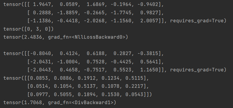
（4）用法

# Example of target with class indices

loss = nn.CrossEntropyLoss()

input = torch.randn(3, 5, requires_grad=True)

target = torch.empty(3, dtype=torch.long).random_(5)

output = loss(input, target)

output.backward()

print(input, target, output, sep='\n')

print('')

# Example of target with class probabilities

input = torch.randn(3, 5, requires_grad=True)

target = torch.randn(3, 5).softmax(dim=1)

output = loss(input, target)

output.backward()

print(input, target, output, sep='\n')

结果：

参考资料

1、PyTorch官方文档

2、【Pytorch系列】nn.BatchNorm2d用法详解