Fuzzy Probability Theory---(2)Computing Fuzzy Probabilities

Let $X=\{x_1,x_2,...,x_n\}$ be a finite set and let $P$ be a probability function defined on all subsets of $X$ with $P(\{x_i\})=a_i,~1\leq i \geq n,~0<a_i<1$ for i and $\sum^{n}_{i=1}=1$. $X$ together with $P$ is a discrete (finite) probability distribution. Now substitue a real number $a_i$ with a fuzzy number $0<\bar{a}_i<1$. If an $a_i$ is crisp, then we will still write it as a fuzzy number even though this fuzzy number is crisp. Then $X$ together with the $\bar{a}_i$ values is a discrete (finite) fuzzy probability distribution. We write $\bar{P}$ for fuzzy $P$ and we have $\bar{P}(\{x_i\})=\bar{a}_i$.

The uncertainty is in some of the $a_i$ values but we know that we have a discrete probability distribution. So we now put the following restriction on the $\bar{a}_i$ values: there are $a_i\in \bar{a}[1]$ so that $\sum^{n}_{i=1}=1$. That is, we can choose $a_i$ in $\bar{a}[\alpha]$ for all $\alpha$, so that we get a discrete probability distribution.

Fuzzy Probability

Suppose $A=\{x_1,x_2,...,x_k\},~1 \leq k < n$. Because $\alpha$-cuts plus interval arithmetic is a feasible way to compute $\bar{P}(A)$, we first need to compute $\bar{P}(A)[\alpha]$ which is $$\bar{P}(A)[\alpha]=\{\sum^{k}_{i=1}a_i~|~S\}$$ where $S$ stands for $a_i\in \bar{a}_i[\alpha], 1\leq i \leq n,~\sum^{n}_{i=1}a_i=1$.

There are 2 constraints on n-dim vector $\vec{a}=(a_1,a_2,...,a_n)$. The first constraint is $\{\sum^{n}_{i=1}a_i=1,~a_i \geq 0\}$ which forms a n-dim subspace $M$, the second constraint is $\{a_i \in \bar{a}_i[\alpha],~1 \leq i \leq n\}$ which also forms a n-dim subspace $N$. Therefore, the elements in $\bar{P}(A)[\alpha]$ can only reside in $Dom[\alpha]=M \cap N$.

There are several properties:

(1)if $A\cap B=\emptyset$, then $\bar{P}(A)+\bar{P}(B) \geq \bar{P}(A\cup B)$.

(2)if $A\cap B \neq \emptyset$, then $\bar{P}(A)+\bar{P}(B)-\bar{P}(A\cap B)\geq \bar{P}(A\cup B)$.

(3)if $A\subseteq B$ and $\bar{P}(A)[\alpha]=[p_{a1}(\alpha),p_{a2}(\alpha)]$ and $\bar{P}(B)[\alpha]=[p_{b1}(\alpha),p_{b2}(\alpha)]$, then $p_{ai}(\alpha)\leq p_{bi}(\alpha)$ for $i=1,2$.

(4)$0\leq \bar{P}(A) \leq 1$ all $A$ with $\bar{P}(\emptyset)=0,~\bar{P}(X)=1$, crisp "one".

(5)$\bar{P}(A)+\bar{P}(A^{'})\geq 1$, crisp "one", where $A^{'}$ is the complement of $A$.

It is easy to see that (3) and (4) are true. (5) is also easy to be seen true if (1) and (2) are true. Now let's demostrate (1) and (2) are really true. First, let's prove (2) is true: Assume $A=\{x_1,x_2,...,x_k\}$, $B=\{x_l,...,x_m\},~for~1 \leq l < k < m <n$

$(2)~is~true\Leftrightarrow (\bar{P}(A)+\bar{P}(B)-\bar{P}(A\cap B))[\alpha] \supseteq \bar{P}(A\cup B)[\alpha]~is~true$

$\Leftrightarrow \bar{P}(A)[\alpha]+\bar{P}(B)[\alpha]-\bar{P}(A\cap B)[\alpha] \supseteq \bar{P}(A\cup B)[\alpha]~is~true$

$\Leftrightarrow \{\sum^{k}_{i=1}a_i~|~S\}+  \{\sum^{m}_{i=l}a_i~|~S\} - \{\sum^{k}_{i=l}a_i~|~S\}   \supseteq  \{\sum^{m}_{i=1}a_i~|~S\}  ~is~true$

Suppose $r$ is a element in $\{\sum^{m}_{i=1}a_i~|~S\}$, then decompose $r=s+t-u$ where $s=\sum^{k}_{i=1}a_i,~t=\sum^{m}_{i=l}a_i,~u=\sum^{k}_{i=l}a_i$. We can see that $s,t,u$ belong respectively to the 1st, 2nd, 3rd member on the left side of equation. Hence $r$ belongs to the left side of equation.

Linear Programming and $\bar{P}(A)$ Computation

Before talking about this topic, let's review what we have learned about LP in our high school. Find numbers $x_1$ and $x_2$ that maximize the sum $x_1+x_2$ subject to $x_1,~x_2\geq 0$, and $$x_1+2x_2\leq 4$$ $$2x_1+x_2\leq 6$$ $$-x_1+x_2 \leq 1$$. And we learned that we first need to draw the feasible area which looks like

Then look at the $x_1+x_2$, move the line of the objective function to get optimal point shown above.

A linear programming problem may be defined as the problem of maximizing or minimizing a linear function subject to linear constraints. The constraints may be equalities or inequalities.  Assume $X=\{x_1,x_2,x_3,x_4,x_5\}$ and $A=\{x_2, x_3,x_4\}$,  then  computing $\bar{P}(A)[\alpha]=\{a_2+a_3+a_4~|~\sum^{5}_{i=1}a_i=1,~a_i \in \bar{a}_i[\alpha],~i=1,2,3,4,5\}$ is a LP problem. That is

Objective Function	$a_2+a_3+a_4$
Main Constraints	$\sum^{5}_{i=1}a_i=1$ $a_i \in \bar{a}_i[\alpha],~i=1,2,3,4,5$
Hidden Constraints	$a_i \geq 0,~i=1,2,3,4,5$
Notation	$\alpha \in [0,1]$

When $\alpha$ is fixed, then $\bar{a}_i[\alpha]$ is fixed. Thus, we can use simplex related method(the basic method in LP) to get the max/min of $(a_2+a_3+a_4)$. A LP library can help us to achieve this without delving into the linear programming optimization methods. We use oscar-linprog, a LP component of OscaR which is a Scala toolkit for solving Operations Research problems. Now Let's do it!

Linear programming using OScaR-Linprog in Eclipse

(1)install sbt

sbt is a build tool for Scala, Java, and more. It requires Java 1.6 or later. Ubuntu 16 has default sbt installed. Since my OS is Ubuntu 16, I don't need to install it.

(2)download oscar from bitbuckit.

I plan to put the cloned code in /home/chase/Projects/FuzzyProbabilities/, then enter into this dir, do

sudo apt install mercurial
hg clone https://bitbucket.org/oscarlib/oscar-releases

(4)start sbt

Start sbt in your terminal with the parameter defining your OS (replace YOUROS by macos64, linux64, win32, win64 according to your OS). My OS is linux64, so get into /home/chase/Projects/FuzzyProbabilities/oscar-releases/oscar-linprog, do

sbt 

After this, sbt will download necessary packages. Finally do

>>eclipse

(4)Download Eclipse with Scala plugin and import the project into Eclipse

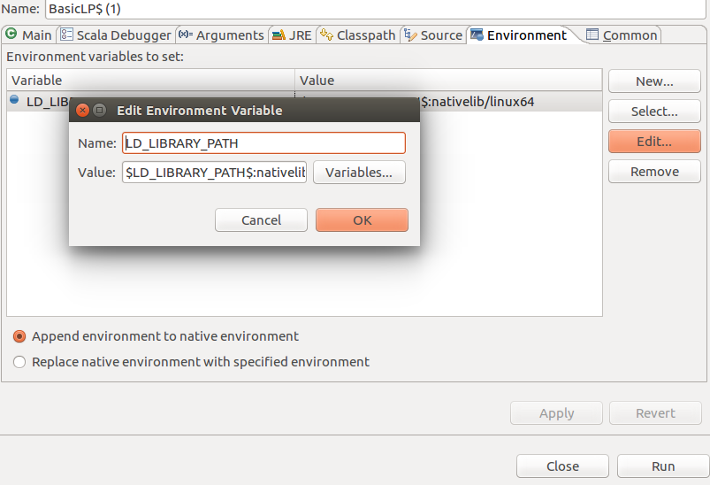
Before you run an application, make sure native libraries have been linked. To do this, right click the main entry -->Run-->Run configuration-->Environment-->New then enter like this

How to compute $\bar{P}(A)$ in a computer?

We know that $\bar{P}(A)$ is actually a fuzzy number, which can be constructed from $\bar{P}(A)[\alpha]$. So to get $\bar{P}(A)$ we first need to get $\bar{P}(A)[\alpha]$. At the same time, we know that $\bar{P}(A)[\alpha]=\{\sum^{k}_{i=1}a_i~|~S\}$ on the assumption that $A=\{x_1,x_2,...,x_k\}$, which, Wow, is just a LP problem where the objective function $ObjFunc=\sum^{k}_{i=1}a_i$ subject to $S$. That is $$\bar{P}(A)[\alpha]=[min\{ObjFunc(\alpha)),max(ObjFunc(\alpha)\}]$$. Therefore we can use the above OscaR-LinPro to compute $\bar{P}(A)[\alpha]$ by which the $\bar{P}(A)$ can be constructed. Note that $\bar{P}(A)$ can only be descretedly approximated by setting $\alpha=[0.01,0.02,0.03,...,0.99,1]$.

Example One

Let $n=5,~A=\{x_1,x_2\},~B=\{x_4,x_5\}$ where $\bar{a}_1=\bar{a}_2=\bar{a}_4=\bar{a}_5=(0.19,0.2,0.21)$, $\bar{a}_3=0.2$. We can see that $A\cap B=\emptyset$. Then $$\bar{P}(A)[\alpha]= \{a_1+a_2~|~S\}=[(19+\alpha)/50,(21-\alpha)/50]$$ and $$\bar{P}(B)[\alpha]=\{a_4+a_5~|~S\}=[(19+\alpha)/50,(21-\alpha)/50]$$. Therefore $$(\bar{P}(A)+\bar{P}(B))[\alpha]=\bar{P}(A)[\alpha]+\bar{P}(B)[\alpha]=[(19+\alpha)/25,(21-\alpha)/25]$$

$\bar{P}(A\cup B)[\alpha]=\{a_1+a_2+a_3+a_4~|~S\}$, since $\sum^{5}_{i=1}a_i=1$ and $a_3=0.2$, hence $a_1+a_2+a_3+a_4$ always persist at 0.8, so $$\bar{P}(A\cup B)[\alpha]=[0.8,0.8]$$. Therefore $\bar{P}(A\cup B)[\alpha] \subseteq (\bar{P}(A)+\bar{P}(B))[\alpha]$, which means $$\bar{P}(A\cup B)<\bar{P}(A)+\bar{P}(B)$$.

Example Two

Let $n=6,~A=\{x_1,x_2,x_3\},~B=\{x_3,x_4,x_5\}$ where $\bar{a}_i=(0.05,0.1,0.15)~where~0 \leq i \leq 5$, also $\bar{a}_6=(0.25,0.5,0.75)$. We can see that $A\cap B\neq \emptyset$. Then $$\bar{P}(A\cup B)[\alpha]=\{\sum^{5}_{i=1}a_i~|~S\}$$

Notation

这里有一个问题，那就是：为什么$\bar{P}(A)$的计算需要LP，而三角模糊数的加减乘除却不需要呢？原因在于前者多了一个限制，即$\sum^{n}_{i=1}a_i=1$,而后者没有这个限制，可以直接用interval arithmetic。

Computing Expectations and Variances

$X=\{x_1,x_2,...,x_n\}$ where $\bar{P}(\{x_i\})=\bar{a}_i,~i=1,2,...,n$. The fuzzy expectation is defined by its $\alpha$-cut $$\bar{u}[\alpha]=\{\sum^{n}_{i=1}x_ia_i~|~S\}$$. The fuzzy variance is defined by its $\alpha$-cut as $$\bar{\sigma}^2[\alpha]=\{\sum^{n}_{i=1}(x_i-u)^2a_i~|~S,~u=\sum^{n}_{i=1}x_ia_i\}$$. $\bar{\sigma}^2$ and $\bar{u}$ are both fuzzy numbers because they are closed, bounded, intervals for $0\leq \alpha \leq 1$.

Example

Let $X=\{0,1,2,3,4\}$ with $a_0=a_4=1/16,~a_2=3/8$ and $\bar{a}_1=\bar{a}_3=(0.2,0.25,0.3)$. First let's compute $\bar{u}$ by its $\alpha$-cut as $$\bar{u}[\alpha]=\{\sum^{4}_{i=0}x_ia_i~|~S\}=\{a_1+2*a_2+3*a_3+4*a_4~|~S\}=\{a_1+3/4+a_3+1/4~|~S\}=\{1+a_1+3*a_3~|~S\}$$. Since $a_1+a_3=1-a_0-a_2-a_4=0.5$, so $a_3=0.5-a_1$, hence the objective function becomes $2.5-2a_1$ which only involves $a_1$, at the same time $a_1\in \bar{a}[\alpha]=[0.2+0.05\alpha,0.3-0.05\alpha]$, so $$\bar{u}[\alpha]=2.5-2[0.2+0.05\alpha,0.3-0.05\alpha]=[2.5,2.5]-[0.4+0.2\alpha,0.6-0.1\alpha]=[1.9+0.1\alpha,2.1-0.1\alpha]$$, so that $\bar{u}[\alpha]=(1.9,2,2.1)$.

Now let's compute $\bar{\sigma}^2$ by its $\alpha$-cut as(note that $u=2.5-2a_1$) $$\bar{\sigma}^2[\alpha]=\{\sum^{4}_{i=0}(x_i-u)^2a_i~|~S,~u=\sum^{4}_{i=0}x_ia_i\}=\{\sum^{4}_{i=0}(x_i+2a_1-2.5)^2a_i~|~S\}=\{-4a^2_1+2a_1+0.75~|~S\}$$. If we analyze this $\bar{\sigma}^2[\alpha]$, we can see that it is a non-linear programming problem because the objective function is non-linear. However, since there is only one variable that affects the objective function $-4a^2_1+2a_1+0.75$ which is a quadratic function with the image shown below. Its central axis is $x=0.25$

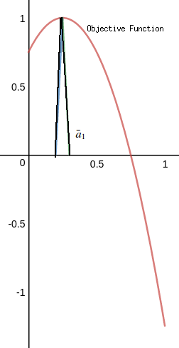
After checking the graph above, we can see that for any $\alpha \in [0,1]$, $\bar{u}^2[\alpha]=[0.99+0.02\alpha-0.01\alpha^2,1]$.

It can be computationally difficult, in general, to compute the intervals $\bar{P}(A)[\alpha],~\bar{u}[\alpha]$(Linear Programming Problems) and $\bar{\sigma}^2[\alpha]$(Non-linear Programming Problems).  One may consider a directed search algorithm (genetic, evolutionary) to estimate $\bar{\sigma}^2[\alpha]$ for a fixed $\alpha$. Rather surprisingly, it turns out that the problem of computing the exact range for the variance over interval data is, in general, NP-hard which means, crudely speaking, that the worst-case computation time grows exponentially with n.

How to compute $\bar{E}$ and $\bar{u}$ of $X$ in a computer?

Very similar, computing $\bar{E}$ and $\bar{u}$ is just like the procedures of computing $\bar{P}$, except that $\bar{u}$ is a non-linear programming problem which is remained to be studied by me.

Fuzzy Conditional Probability

Let $A=\{x_1,x_2,...,x_k\}$ and $B=\{x_l,...,x_m\}$ where $1\leq l \leq k \leq m \leq n$ so that A and B are not disjoint. So $$\bar{P}(A|B)=\{\frac{\sum^{k}_{i=l}a_i}{\sum^{m}_{i=l}a_i}|~S~\}$$. We know that in crisp sets, $P(A|B)=P(A\cup B)/P(B)$. Naturally we might define $\bar{P}(A|B)=\bar{P}(A\cup B)/\bar{P}(B)$ however it can get outside of interval [0,1] so we don't use this. Then is the properties of $\bar{P}(A|B)$ similar to that of the crisp $\bar{P}(A|B)$? NO!

(1) $0 \leq \bar{P}(A|B) \leq 1$

(2) $\bar{P}(B|B)=1$

(3) $\bar{P}(A|B)=1$ if $B\in A$

(4) $\bar{P}(A|B)=0$ if $B \cap A = \emptyset$

(5) $\bar{P}(A_1 \cup A_2 | B) \leq \bar{P}(A_1|B)+\bar{P}(A_2|B)$, if $A_1 \cap A_2= \emptyset$

Fuzzy Independence

A and B are strongly independent if $$\bar{P}(A|B)=\bar{P}(A)~and~\bar{P}(B|A)=\bar{P}(B)$$. Since strongly independent is difficult to satisfy we also have a weaker definition of independence. A and B are weakly independent if $$\bar{P}(A|B)[1]=\bar{P}(A)[1]~and~\bar{P}(B|A)[1]=\bar{P}(B)[1]$$. Clearly, if A and B are strongly independent they are weakly independent. In crisp situation, we know A and B are independent if $P(A\cap B)=P(A)P(B)$. But this is not that suitable for fuzzy situations because $\bar{P}(A\cap B)=\bar{P}(A)\bar{P}(B)$ is extremely hard to satisfy.

Fuzzy Bayes' Formula

Let $A_i,~1\leq i \leq m$ be a partition of $X=\{x_1,x_2,...,x_n\}$. That is, the $A_i$ are non-empty, mutually disjoint and thier unions are $X$. There is a finite set of chance events, also called the states of nature, $S=\{S_1,...,S_k\}$. We don't know $P(A_i)$ but we do know $$a_{ik}=P(A_i|S_k)$$ where $1\leq i \leq m,~1\leq k \leq K$. That is, if we know $S_k$, then $a_{ik}$ give the probabilities of the events $A_i$.

We invite a group of experts to estimate $a_k=P(S_k)$ which is called the prior probability distribution over the states of nature. Predictably, the estimated $P(S_k)$ may be far away from the god truth, so what we do is to update $P(S_k)$ after a $A_i$ has occurred. We use the following formulation to describe the above process:

Let us see how this result may be used. Using the $a_{ik}$ and the prior distribution $a_k$, we may calculate $P(A_i)$ as follows $$P(A_i)=\sum^{K}_{k=1}P(A_i|S_k)P(S_k)$$. Now we gather information and observe that event $A_j$ has occurred. We update the prior to the posterior and then obtain improved estimates of the probabilities for the $A_i$ as

Now substitute $\bar{a}_k$ for $a_k$, $1\leq k\leq K$. Suppose we observe that event $A_j$ has occurred. $\alpha$-cuts of the fuzzy posterior distribution are $$\bar{P}(S_k|A_j)[\alpha]=\{\frac{a_{jk}a_k}{\sum^{K}_{k=1}a_{jk}a_k}~|~S\}$$ where $S$ is the statement $a_k\in \bar{a}_k[\alpha],~1\leq k \leq K,~ \sum^{K}_{k=1}a_k=1$. Once we have the fuzzy posterior, we may update our fuzzy probability for the $A_j$.

3 Parameter Estimators

In crisp sets, there are 3 methods for training/estimating parameters of a probabilistic model $p(x;\theta)$ from which data set $X$ have been observed.

ML(Maximun Likelihood) estimator: $\theta_{ML}=argmax~p(X|\theta)$

MAP(Maximun a Posterior) estimator: $\theta_{MAP}=argmax~p(\theta|X)=argmax~p(X|\theta)p(\theta)$

Bayes estimator: $\theta_{Bayes}=E[\theta|X]=\int \theta p(\theta|X) d\theta$

No matter which method we take, we can use the estimated $\theta$ to estimate the density at $x_0$. That is

$$p(x_0|X)=\int p((x_0,\theta)|X) d\theta=\int p(x_0|\theta, X) p(\theta|X)d\theta=\int p(x_0|\theta) p(\theta|X)d\theta$$ where $p(x_0|\theta)=p(x_0|\theta,X)$ because because once we know $\theta$, the sufficient statistics, we know everything about the distribution. Thus we are taking an average on $p(x_0|\theta)$ using all values of θ, weighted by their probabilities $p(\theta|X)$. However evaluating the integrals may be quite difficult except in cases where the posterior has a nice form. So we reduce it to a single point, for example, using MAP to make the calculation easier: $\theta_{MAP}=argmax~p(\theta|X)$. Then how about the 3 corresponding fuzzy parameter estimaters? I will come back later when I go through continuous fuzzy random variables.

Applications

In this section we will use $p_i$ for probability values instead of $a_i$.

Blood Types

There are four basic blood types: A, B, AB and O. Qingdao conducted a random sample of 1000 people from the pool of blood donors and they determine the following point estimates: $p_a=0.33,~p_b=0.23,~p_{ab}=0.35,~p_o=0.09$. Because these are point estimates based on a random sample, we will substitute fuzzy numbers for these probabilities. Let $\bar{p}_a=(0.3,0.33,0.36),\bar{p}_b=0.2,0.23,0.26,\bar{p}_{ab}=(0.32,0.35,0.38),\bar{p}_o=(0.06,0.09,0.12)$. Next let $\bar{P}(O^{'})$ stands for the fuzzy probability of a donor not having blood type O. We know from the above sections that $\bar{P}(O)+\bar{P}(O^{'})\geq 1$, so we can only compute its $\alpha$-cuts as $$\bar{P}(O^{'})[\alpha]=\{p_a+p_b+p_{ab}~|~S\}$$ where $S$ means $p_a \in \bar{p}_a[\alpha],~p_b \in \bar{p}_b[\alpha],~p_{ab} \in \bar{p}_{ab}[\alpha], p_o\in \bar{p}_o[\alpha],~p_a+p_b+p_{ab}+p_o=1$. Then use OscaR Linpro to compute $\bar{P}(O^{'})[\alpha],~\alpha=0,0.2,0.4,0.8,1$, we get

The code is

Resistance to Surveys

There are young people and old people, and there are people willing to answer a survey and people resisting to answer a survey. 18%($p_1$) of young people said they will respond to questions in a survey while 5%(p_2) young people said they would. 68%($p_3$) of the older people responded that they would participate in a survey while 9%($p_4$) of them said theu would not. Now choosing at random one person from this group, then what is the probability that this person is young or is someone who would refuse to respond to the questions in a survey?

All these probabilities were estimated and so we substitute fuzzy numbers for the $p_i$. Assume that we decide to use: (1) $\bar{p}_1=(0.16/0.18/0.2)$ for $p_1$ (2) $\bar{p}_2=(0.03/0.05/0.07)$ for $p_2$ (3) $\bar{p}_3=(0.61/0.68/0.75)$ for $p_3$ (4) $\bar{p}_3=(0.07/0.09/0.11)$ for $p_4$. set $A=\{young people, old people\},B=\{respond to surveys, refuse surveys\}$, then we can see that the joint probability distribution P(A,B)=\{p_1,p_2,p_3,p_4\}. What we want to compute is $P(A \cup B_2)=\{p_1+p_2+p_4~|~S\}$ where $S$ means $p_i \in \bar{p}_i[\alpha], 1\leq i \leq 4,~ and p_1+p_2+p_3+p_4=1$.

Testing for HIV

$A_1$: a person is infected with HIV. $A_2$: a person is not infected with HIV. $B_1$: a person is tested "positive". $B_2$: a person is tested "negative". We want to find $\bar{P}(A_1|B_1)$. We denote $P(A_1\cap B_1)=p_{11},~P(A_1\cap B_2)=p_{12},~P(A_2\cap B_1)=p_{21},~P(A_2\cap B_2)=p_{22}$. We know that $$P(A_1|B_1)=\frac{P(A_1\cap B_1)}{P(B_1)}=\frac{P(B_1\cap A_1)}{P(A_1\cap B_1)+P(A_2\cap B_1)}=\frac{p_{11}}{p_{11}+p_{21}}$$. Therefore the fuzzy version becomes $$\bar{P}(A_1|B_1)[\alpha]=\{\frac{p_{11}}{p_{11}+p_{21}}~|~S\}$$ where $S$ means $p_{ij} \in \bar{p}_{ij}[\alpha]$ and all the $p_{ij}$ must be equal to one. This is a non-linear programming problem.

Fuzzy Bayes

Let's see how $\bar{P}(A_1)$ changes from the fuzzy prior to the fuzzy posterior. Suppose the nature random variable $S$ only takes two states, $S_1$ and $S_2$ with fuzzy prior probability $\bar{p}_1=\bar{P}(S_1)=(0.3/0.4/0.5)$ and $\bar{p}_2=\bar{P}(S_2)=(0.5/0.6/0.7)$. Two events $A_1$ and $A_2$ partition $X$ with known conditional probabilities $p_{11}=P(A_1|S_1)=0.2,~p_{21}=P(A_2|S_1)=0.8,~p_{12}=P(A_1|S_2)=0.7,~p_{22}=P(A_2|S_2)=0.3$. We first find the fuzzy probability $\bar{P}(A_1)$ using the fuzzy prior probabilities. Its $\alpha$-cuts are $$\bar{P}(A_1)[\alpha]=\{0.2p_1+0.7p_2~|~S\}$$ where $S$ means $p_1\in \bar{p}_1[\alpha],~p_2\in \bar{p}_2[\alpha],~p_1+p_2=1$. Now the the $$\bar{P}(A_1)=(0.41/0.5/0.59)$$.

The $\bar{P}(A_1)$ above is an old version, now we want to update it using Fuzzy Bayes. To update $\bar{P}(A_1)$ we need first update $\bar{P}(S_1|A_1),~\bar{P}(S_2|A_1)$. Now lets do it! $$\bar{P}(S_1|A_1)[\alpha]=\{\frac{0.2p_1}{0.2p_1+0.7p_2}~|~S\}~~\bar{P}(S_2|A_1)[\alpha]=\{\frac{0.7p_2}{0.2p_1+0.7p_2}~|~S\}$$ where $S$ is $p_i \in \bar{p}_i[\alpha], i=1,2，~p_1+p_2=1$. We get

Now we may compute the new $\bar{P}(A_1)$, which is $$\bar{P}(A_1)[\alpha]=\{0.2p_1+0.7p_2~|~S\}$$ where $S$ is $p_1\in \bar{P}(S_1|A_1)[\alpha],~p_2\in \bar{P}(S_2|A_1)[\alpha],~p_1+p_2=1$