基于theano的多层感知机的实现
1.引言
一个多层感知机(Multi-Layer Perceptron,MLP)可以看做是,在逻辑回归分类器的中间加了非线性转换的隐层,这种转换把数据映射到一个线性可分的空间。一个单隐层的MLP就可以达到全局最优。
2.模型
一个单隐层的MLP可以表示如下:

一个隐层的MLP是一个函数:$f:R^{D}\rightarrow R^{L}$,其中 $D$ 是输入向量 $x$ 的大小,$L$是输出向量 $f(x)$ 的大小:
$f(x)=G(b^{(2)}+W^{(2)}(s(b^{(1)}+W^{(1)}))),$
向量$h(x)=s(b^{(1)}+W^{(1)})$构成了隐层,$W^{(1)}\in R^{D\times D_{h}}$ 是连接输入和隐层的权重矩阵,激活函数$s$可以是 $tanh(a)=(e^{a}-e^{-a})/(e^{a}+e^{-a})$ 或者 $sigmoid(a)=1/(1+e^{-a})$,但是前者通常会训练比较快。
在输出层得到:$o(x)=G(b^{(2)}+W^{(2)}h(x))$
为了训练MLP,所有参数 $\theta=\{W^{(2)},b^{(2)},W^{(1)},b^{\text{(1)}}\}.$ 用随机梯度下降法训练,参数的求导用反向传播算法来求。这里在顶层分类的时候用到了前面的逻辑回归的代码:
Python学习笔记之逻辑回归.
3.从逻辑回归到MLP
这里以单隐层MLP为例,当把数据由输入层映射到隐层之后,再加上一个逻辑回归层就构成了MLP.
 class HiddenLayer(object):

     def __init__(self, rng, input, n_in, n_out, W=None, b=None,

                  activation=T.tanh):

         """

         Typical hidden layer of a MLP: units are fully-connected and have

         sigmoidal activation function. Weight matrix W is of shape (n_in,n_out)

         and the bias vector b is of shape (n_out,).

         NOTE : The nonlinearity used here is tanh

         Hidden unit activation is given by: tanh(dot(input,W) + b)

         :type rng: numpy.random.RandomState

         :param rng: a random number generator used to initialize weights

         :type input: theano.tensor.dmatrix

         :param input: a symbolic tensor of shape (n_examples, n_in)

         :type n_in: int

         :param n_in: dimensionality of input

         :type n_out: int

         :param n_out: number of hidden units

         :type activation: theano.Op or function

         :param activation: Non linearity to be applied in the hidden

                            layer

         """

         self.input = input
权重的初始化依赖于激活函数,根据[Xavier10]证明显示,对于$tanh$激活函数,权重初始值应该从$[-\sqrt{\frac{6}{fan_{in}+fan_{out}}},\sqrt{\frac{6}{fan_{in}+fan_{out}}}]$区间内均匀采样得到,其中 $fan_{in}$ 是第$(i-1)$ 层的单元数量,$fan_{out}$ 是第 $i$ 层的单元数量,对于sigmoid函数,采样区间应该变为 $[-4\sqrt{\frac{6}{fan_{in}+fan_{out}}},4\sqrt{\frac{6}{fan_{in}+fan_{out}}}]$.这种初始化方式能保证在训练的初始阶段,通过激活函数能够使得信息有效地向上和向下传播。
 if W is None:

             W_values = numpy.asarray(

                 rng.uniform(

                     # 随机数位于[low,high)区间

                     low=-numpy.sqrt(6. / (n_in + n_out)),

                     high=numpy.sqrt(6. / (n_in + n_out)),

                     size=(n_in, n_out)

                 ),

                 # 类型设为 floatX 是为了在GPU上运行

                 dtype=theano.config.floatX

             )

             # 如果激活函数是 sigmoid,权重初始化要变大

             if activation == theano.tensor.nnet.sigmoid:

                 W_values *= 4

             # borrow = True 表示数据执行浅拷贝,增加效率

             W = theano.shared(value=W_values, name='W', borrow=True)

         if b is None:

             b_values = numpy.zeros((n_out,), dtype=theano.config.floatX)

             b = theano.shared(value=b_values, name='b', borrow=True)

         self.W = W

         self.b = b

         lin_output = T.dot(input, self.W) + self.b

         self.output = (

             lin_output if activation is None

             else activation(lin_output)

         )

         # parameters of the model

         self.params = [self.W, self.b]
在上面两步的基础上构建MLP:
 class MLP(object):

     """Multi-Layer Perceptron Class

     A multilayer perceptron is a feedforward artificial neural network model

     that has one layer or more of hidden units and nonlinear activations.

     Intermediate layers usually have as activation function tanh or the

     sigmoid function (defined here by a ``HiddenLayer`` class)  while the

     top layer is a softamx layer (defined here by a ``LogisticRegression``

     class).

     """

     def __init__(self, rng, input, n_in, n_hidden, n_out):

         """Initialize the parameters for the multilayer perceptron

         :type rng: numpy.random.RandomState

         :param rng: a random number generator used to initialize weights

         :type input: theano.tensor.TensorType

         :param input: symbolic variable that describes the input of the

         architecture (one minibatch)

         :type n_in: int

         :param n_in: number of input units, the dimension of the space in

         which the datapoints lie

         :type n_hidden: int

         :param n_hidden: number of hidden units

         :type n_out: int

         :param n_out: number of output units, the dimension of the space in

         which the labels lie

         """

         # Since we are dealing with a one hidden layer MLP, this will translate

         # into a HiddenLayer with a tanh activation function connected to the

         # LogisticRegression layer; the activation function can be replaced by

         # sigmoid or any other nonlinear function

         self.hiddenLayer = HiddenLayer(

             rng=rng,

             input=input,

             n_in=n_in,

             n_out=n_hidden,

             activation=T.tanh

         )

         # The logistic regression layer gets as input the hidden units

         # of the hidden layer

         self.logRegressionLayer = LogisticRegression(

             input=self.hiddenLayer.output,

             n_in=n_hidden,

             n_out=n_out

         )
为了防止过拟合,这里加上 L1 和 L2 正则项,即计算权重 $W^{(1)},W^{(2)}$ 的1范数和2范数:
   # L1 norm ; one regularization option is to enforce L1 norm to

         # be small

         self.L1 = (

             abs(self.hiddenLayer.W).sum()

             + abs(self.logRegressionLayer.W).sum()

         )

         # square of L2 norm ; one regularization option is to enforce

         # square of L2 norm to be small

         self.L2_sqr = (

             (self.hiddenLayer.W ** 2).sum()

             + (self.logRegressionLayer.W ** 2).sum()

         )

         # negative log likelihood of the MLP is given by the negative

         # log likelihood of the output of the model, computed in the

         # logistic regression layer

         self.negative_log_likelihood = (

             self.logRegressionLayer.negative_log_likelihood

         )

         # same holds for the function computing the number of errors

         self.errors = self.logRegressionLayer.errors

         # the parameters of the model are the parameters of the two layer it is

         # made out of

         self.params = self.hiddenLayer.params + self.logRegressionLayer.params
似然函数的值加上正则项构成损失函数:
 # the cost we minimize during training is the negative log likelihood of

     # the model plus the regularization terms (L1 and L2); cost is expressed

     # here symbolically

     cost = (

         classifier.negative_log_likelihood(y)

         + L1_reg * classifier.L1

         + L2_reg * classifier.L2_sqr

     )
4.Minist识别测试
"""
This tutorial introduces the multilayer perceptron using Theano. A multilayer perceptron is a logistic regressor where
instead of feeding the input to the logistic regression you insert a
intermediate layer, called the hidden layer, that has a nonlinear
activation function (usually tanh or sigmoid) . One can use many such
hidden layers making the architecture deep. The tutorial will also tackle
the problem of MNIST digit classification. .. math:: f(x) = G( b^{(2)} + W^{(2)}( s( b^{(1)} + W^{(1)} x))), References: - textbooks: "Pattern Recognition and Machine Learning" -
Christopher M. Bishop, section 5 """
__docformat__ = 'restructedtext en' import os
import sys
import time import numpy import theano
import theano.tensor as T from logistic_sgd import LogisticRegression, load_data # start-snippet-1
class HiddenLayer(object):
def __init__(self, rng, input, n_in, n_out, W=None, b=None,
activation=T.tanh):
"""
Typical hidden layer of a MLP: units are fully-connected and have
sigmoidal activation function. Weight matrix W is of shape (n_in,n_out)
and the bias vector b is of shape (n_out,). NOTE : The nonlinearity used here is tanh Hidden unit activation is given by: tanh(dot(input,W) + b) :type rng: numpy.random.RandomState
:param rng: a random number generator used to initialize weights :type input: theano.tensor.dmatrix
:param input: a symbolic tensor of shape (n_examples, n_in) :type n_in: int
:param n_in: dimensionality of input :type n_out: int
:param n_out: number of hidden units :type activation: theano.Op or function
:param activation: Non linearity to be applied in the hidden
layer
"""
self.input = input
# end-snippet-1 # `W` is initialized with `W_values` which is uniformely sampled
# from sqrt(-6./(n_in+n_hidden)) and sqrt(6./(n_in+n_hidden))
# for tanh activation function
# the output of uniform if converted using asarray to dtype
# theano.config.floatX so that the code is runable on GPU
# Note : optimal initialization of weights is dependent on the
# activation function used (among other things).
# For example, results presented in [Xavier10] suggest that you
# should use 4 times larger initial weights for sigmoid
# compared to tanh
# We have no info for other function, so we use the same as
# tanh.
if W is None:
W_values = numpy.asarray(
rng.uniform(
# 随机数位于[low,high)区间
low=-numpy.sqrt(6. / (n_in + n_out)),
high=numpy.sqrt(6. / (n_in + n_out)),
size=(n_in, n_out)
),
# 类型设为 floatX 是为了在GPU上运行
dtype=theano.config.floatX
)
# 如果激活函数是 sigmoid,权重初始化要变大
if activation == theano.tensor.nnet.sigmoid:
W_values *= 4
# borrow = True 表示数据执行浅拷贝,增加效率
W = theano.shared(value=W_values, name='W', borrow=True) if b is None:
b_values = numpy.zeros((n_out,), dtype=theano.config.floatX)
b = theano.shared(value=b_values, name='b', borrow=True) self.W = W
self.b = b lin_output = T.dot(input, self.W) + self.b
self.output = (
lin_output if activation is None
else activation(lin_output)
)
# parameters of the model
self.params = [self.W, self.b] # start-snippet-2
class MLP(object):
"""Multi-Layer Perceptron Class A multilayer perceptron is a feedforward artificial neural network model
that has one layer or more of hidden units and nonlinear activations.
Intermediate layers usually have as activation function tanh or the
sigmoid function (defined here by a ``HiddenLayer`` class) while the
top layer is a softamx layer (defined here by a ``LogisticRegression``
class).
""" def __init__(self, rng, input, n_in, n_hidden, n_out):
"""Initialize the parameters for the multilayer perceptron :type rng: numpy.random.RandomState
:param rng: a random number generator used to initialize weights :type input: theano.tensor.TensorType
:param input: symbolic variable that describes the input of the
architecture (one minibatch) :type n_in: int
:param n_in: number of input units, the dimension of the space in
which the datapoints lie :type n_hidden: int
:param n_hidden: number of hidden units :type n_out: int
:param n_out: number of output units, the dimension of the space in
which the labels lie """ # Since we are dealing with a one hidden layer MLP, this will translate
# into a HiddenLayer with a tanh activation function connected to the
# LogisticRegression layer; the activation function can be replaced by
# sigmoid or any other nonlinear function
self.hiddenLayer = HiddenLayer(
rng=rng,
input=input,
n_in=n_in,
n_out=n_hidden,
activation=T.tanh
) # The logistic regression layer gets as input the hidden units
# of the hidden layer
self.logRegressionLayer = LogisticRegression(
input=self.hiddenLayer.output,
n_in=n_hidden,
n_out=n_out
)
# end-snippet-2 start-snippet-3
# L1 norm ; one regularization option is to enforce L1 norm to
# be small
self.L1 = (
abs(self.hiddenLayer.W).sum()
+ abs(self.logRegressionLayer.W).sum()
) # square of L2 norm ; one regularization option is to enforce
# square of L2 norm to be small
self.L2_sqr = (
(self.hiddenLayer.W ** 2).sum()
+ (self.logRegressionLayer.W ** 2).sum()
) # negative log likelihood of the MLP is given by the negative
# log likelihood of the output of the model, computed in the
# logistic regression layer
self.negative_log_likelihood = (
self.logRegressionLayer.negative_log_likelihood
)
# same holds for the function computing the number of errors
self.errors = self.logRegressionLayer.errors # the parameters of the model are the parameters of the two layer it is
# made out of
self.params = self.hiddenLayer.params + self.logRegressionLayer.params
# end-snippet-3 def test_mlp(learning_rate=0.01, L1_reg=0.00, L2_reg=0.0001, n_epochs=1000,
dataset='mnist.pkl.gz', batch_size=20, n_hidden=500):
"""
Demonstrate stochastic gradient descent optimization for a multilayer
perceptron This is demonstrated on MNIST. :type learning_rate: float
:param learning_rate: learning rate used (factor for the stochastic
gradient :type L1_reg: float
:param L1_reg: L1-norm's weight when added to the cost (see
regularization) :type L2_reg: float
:param L2_reg: L2-norm's weight when added to the cost (see
regularization) :type n_epochs: int
:param n_epochs: maximal number of epochs to run the optimizer :type dataset: string
:param dataset: the path of the MNIST dataset file from
http://www.iro.umontreal.ca/~lisa/deep/data/mnist/mnist.pkl.gz """
datasets = load_data(dataset) train_set_x, train_set_y = datasets[0]
valid_set_x, valid_set_y = datasets[1]
test_set_x, test_set_y = datasets[2] # compute number of minibatches for training, validation and testing
n_train_batches = train_set_x.get_value(borrow=True).shape[0] / batch_size
n_valid_batches = valid_set_x.get_value(borrow=True).shape[0] / batch_size
n_test_batches = test_set_x.get_value(borrow=True).shape[0] / batch_size ######################
# BUILD ACTUAL MODEL #
######################
print '... building the model' # allocate symbolic variables for the data
index = T.lscalar() # index to a [mini]batch
x = T.matrix('x') # the data is presented as rasterized images
y = T.ivector('y') # the labels are presented as 1D vector of
# [int] labels rng = numpy.random.RandomState(1234) # construct the MLP class
classifier = MLP(
rng=rng,
input=x,
n_in=28 * 28,
n_hidden=n_hidden,
n_out=10
) # start-snippet-4
# the cost we minimize during training is the negative log likelihood of
# the model plus the regularization terms (L1 and L2); cost is expressed
# here symbolically
cost = (
classifier.negative_log_likelihood(y)
+ L1_reg * classifier.L1
+ L2_reg * classifier.L2_sqr
)
# end-snippet-4 # compiling a Theano function that computes the mistakes that are made
# by the model on a minibatch
test_model = theano.function(
inputs=[index],
outputs=classifier.errors(y),
givens={
x: test_set_x[index * batch_size:(index + 1) * batch_size],
y: test_set_y[index * batch_size:(index + 1) * batch_size]
}
) validate_model = theano.function(
inputs=[index],
outputs=classifier.errors(y),
givens={
x: valid_set_x[index * batch_size:(index + 1) * batch_size],
y: valid_set_y[index * batch_size:(index + 1) * batch_size]
}
) # start-snippet-5
# compute the gradient of cost with respect to theta (sotred in params)
# the resulting gradients will be stored in a list gparams
gparams = [T.grad(cost, param) for param in classifier.params] # specify how to update the parameters of the model as a list of
# (variable, update expression) pairs # given two list the zip A = [a1, a2, a3, a4] and B = [b1, b2, b3, b4] of
# same length, zip generates a list C of same size, where each element
# is a pair formed from the two lists :
# C = [(a1, b1), (a2, b2), (a3, b3), (a4, b4)]
updates = [
(param, param - learning_rate * gparam)
for param, gparam in zip(classifier.params, gparams)
] # compiling a Theano function `train_model` that returns the cost, but
# in the same time updates the parameter of the model based on the rules
# defined in `updates`
train_model = theano.function(
inputs=[index],
outputs=cost,
updates=updates,
givens={
x: train_set_x[index * batch_size: (index + 1) * batch_size],
y: train_set_y[index * batch_size: (index + 1) * batch_size]
}
)
# end-snippet-5 ###############
# TRAIN MODEL #
###############
print '... training' # early-stopping parameters
patience = 10000 # look as this many examples regardless
patience_increase = 2 # wait this much longer when a new best is
# found
improvement_threshold = 0.995 # a relative improvement of this much is
# considered significant
validation_frequency = min(n_train_batches, patience / 2)
# go through this many
# minibatche before checking the network
# on the validation set; in this case we
# check every epoch best_validation_loss = numpy.inf
best_iter = 0
test_score = 0.
start_time = time.clock() epoch = 0
done_looping = False
# 迭代 n_epochs 次,每次迭代都将遍历训练集所有样本
while (epoch < n_epochs) and (not done_looping):
epoch = epoch + 1
for minibatch_index in xrange(n_train_batches): minibatch_avg_cost = train_model(minibatch_index)
# iteration number
iter = (epoch - 1) * n_train_batches + minibatch_index # 训练一定的样本之后才进行交叉验证
if (iter + 1) % validation_frequency == 0:
# compute zero-one loss on validation set
validation_losses = [validate_model(i) for i
in xrange(n_valid_batches)]
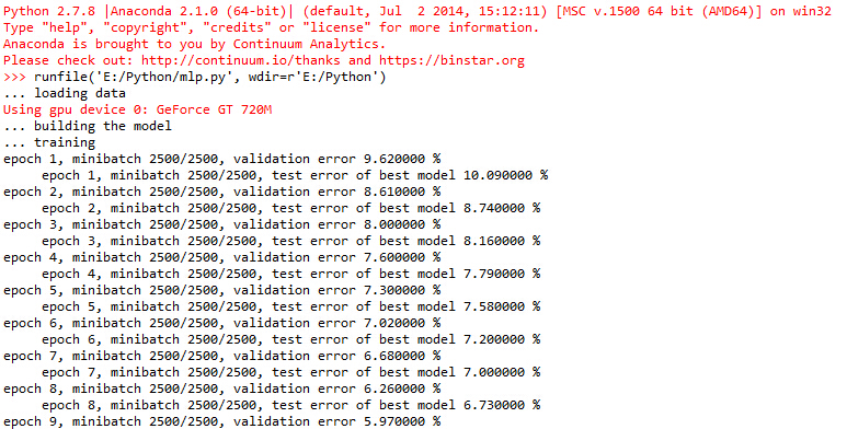
this_validation_loss = numpy.mean(validation_losses) print(
'epoch %i, minibatch %i/%i, validation error %f %%' %
(
epoch,
minibatch_index + 1,
n_train_batches,
this_validation_loss * 100.
)
) # if we got the best validation score until now
# 如果交叉验证的误差比当前最小的误差还小,就在测试集上测试
if this_validation_loss < best_validation_loss:
# improve patience if loss improvement is good enough
# 如果改善很多,就在本次迭代中多训练一定数量的样本
if (
this_validation_loss < best_validation_loss *
improvement_threshold
):
patience = max(patience, iter * patience_increase) # 记录最小的交叉验证误差和相应的迭代数
best_validation_loss = this_validation_loss
best_iter = iter # test it on the test set
test_losses = [test_model(i) for i
in xrange(n_test_batches)]
test_score = numpy.mean(test_losses) print((' epoch %i, minibatch %i/%i, test error of '
'best model %f %%') %
(epoch, minibatch_index + 1, n_train_batches,
test_score * 100.))
# 训练样本数超过 patience,即停止
if patience <= iter:
done_looping = True
break end_time = time.clock()
print(('Optimization complete. Best validation score of %f %% '
'obtained at iteration %i, with test performance %f %%') %
(best_validation_loss * 100., best_iter + 1, test_score * 100.))
print >> sys.stderr, ('The code for file ' +
os.path.split(__file__)[1] +
' ran for %.2fm' % ((end_time - start_time) / 60.)) if __name__ == '__main__':
test_mlp()
关于上面代码中的交叉验证:只有训练结果的交叉验证结果比上一次交叉验证结果好,才在测试集上进行测试!
训练过程截图:
学习内容来源:
http://deeplearning.net/tutorial/mlp.html#mlp
基于theano的多层感知机的实现的更多相关文章
- Theano3.4-练习之多层感知机
来自http://deeplearning.net/tutorial/mlp.html#mlp Multilayer Perceptron note:这部分假设读者已经通读之前的一个练习 Classi ...
- (数据科学学习手札44)在Keras中训练多层感知机
一.简介 Keras是有着自主的一套前端控制语法,后端基于tensorflow和theano的深度学习框架,因为其搭建神经网络简单快捷明了的语法风格,可以帮助使用者更快捷的搭建自己的神经网络,堪称深度 ...
- DeepLearning tutorial(3)MLP多层感知机原理简介+代码详解
本文介绍多层感知机算法,特别是详细解读其代码实现,基于python theano,代码来自:Multilayer Perceptron,如果你想详细了解多层感知机算法,可以参考:UFLDL教程,或者参 ...
- MLP多层感知机
@author:wepon @blog:http://blog.csdn.net/u012162613/article/details/43221829 转载:http://blog.csdn.net ...
- (数据科学学习手札34)多层感知机原理详解&Python与R实现
一.简介 机器学习分为很多个领域,其中的连接主义指的就是以神经元(neuron)为基本结构的各式各样的神经网络,规范的定义是:由具有适应性的简单单元组成的广泛并行互连的网络,它的组织能够模拟生物神经系 ...
- TensorFlow学习笔记7-深度前馈网络(多层感知机)
深度前馈网络(前馈神经网络,多层感知机) 神经网络基本概念 前馈神经网络在模型输出和模型本身之间没有反馈连接;前馈神经网络包含反馈连接时,称为循环神经网络. 前馈神经网络用有向无环图表示. 设三个函数 ...
- Alink漫谈(十四) :多层感知机 之 总体架构
Alink漫谈(十四) :多层感知机 之 总体架构 目录 Alink漫谈(十四) :多层感知机 之 总体架构 0x00 摘要 0x01 背景概念 1.1 前馈神经网络 1.2 反向传播 1.3 代价函 ...
- Alink漫谈(十五) :多层感知机 之 迭代优化
Alink漫谈(十五) :多层感知机 之 迭代优化 目录 Alink漫谈(十五) :多层感知机 之 迭代优化 0x00 摘要 0x01 前文回顾 1.1 基本概念 1.2 误差反向传播算法 1.3 总 ...
- Tensorflow 2.0 深度学习实战 —— 详细介绍损失函数、优化器、激活函数、多层感知机的实现原理
前言 AI 人工智能包含了机器学习与深度学习,在前几篇文章曾经介绍过机器学习的基础知识,包括了监督学习和无监督学习,有兴趣的朋友可以阅读< Python 机器学习实战 >.而深度学习开始只 ...
随机推荐
- c++ 读写功能
课程作业三 git链接: Operations 感想 这次代码修改的地方主要有,加入了文件读写.读出功能,以及分离函数写到了头文件里. 但是也有很多不足的地方,首先本来想要 ...
- 回忆--RYU流量监控
RYU流量监控 前言 Ryu book上的一个流量监控的应用,相对比较好看懂 实验代码 github源码 from ryu.app import simple_switch_13 from ryu.c ...
- 11th 回顾5个问题
当初提出的5个问题: 1.书中说很多非常成功的软件都是赢在用户体验,后面的第12章也专门提到了用户体验,说软件开发时可以使用5W1H的方法来判断用户的体验,而需求分析需要获取用户需求,进行用户调研,那 ...
- 使用Webdriver刷博客文章评论
package com.zhc.webdriver; import java.util.ArrayList; import java.util.Iterator; import java.util.c ...
- SpringMvc+JavaConfig+Idea 基于JavaConfig搭建项目
1.介绍 之前搭建SpringMvc项目要配置一系列的配置文件,比如web.xml,applicationContext.xml,dispatcher.xml.Spring 3.X之后推出了基于Jav ...
- TRichEdit怎样新增的内容到最后一行?
Delphi里使用TRichEdit,使用SetSelTextBuf时可以设置显示的字体格式,但是显示位置是在当前的插入光标后,如果人为改变插入光标的位置,比如在其他位置单,以后再插入的内容位置就没办 ...
- Ubuntu17安装MySql5.7
安装: sudo apt-get update sudo apt-get install mysql-server 配置远程访问: vi /etc/mysql/mysql.conf.d/mysqld. ...
- 【设计模式】—— 组合模式Composite
前言:[模式总览]——————————by xingoo 模式意图 使对象组合成树形的结构.使用户对单个对象和组合对象的使用具有一致性. 应用场景 1 表示对象的 部分-整体 层次结构 2 忽略组合对 ...
- 【设计模式】——工厂方法FactoryMethod
前言:[模式总览]——————————by xingoo 模式意图 工厂方法在MVC中应用的很广泛. 工厂方法意在分离产品与创建的两个层次,使用户在一个工厂池中可以选择自己想要使用的产品,而忽略其创建 ...
- call/cc 总结 | Scheme
call/cc 总结 | Scheme 来源 https://www.sczyh30.com/posts/Functional-Programming/call-with-current-contin ...