self attention pytorch代码

实现细节;

1.embedding 层

2.positional encoding层:添加位置信息

3,MultiHeadAttention层:encoder的self attention

4,sublayerConnection层：add&norm，使用layerNorm，

5,FeedForward层:两层全连接

6,Masked MultiHeadAttention:decoder中的self attention层，添加mask,不考虑计算当前位置的后面信息

7,MultiHeadAttention层:encoder的输出做key,value,decoder的self attention输出做query,类似于传统attention

8,generator层:最后的linear和softmax层，转为概率输出

9,预测时greedy_decode,第一个预测初始化为start字符

 #!/usr/bin/env python
 # coding: utf-8

 import numpy as np
 import torch
 import torch.nn as nn
 import torch.nn.functional as F
 import math
 import copy
 import time
 from torch.autograd import Variable
 import matplotlib.pyplot as plt
 import seaborn
 seaborn.set_context(context="talk")

 class EncoderDecoder(nn.Module):
     """
     A standard Encoder-Decoder architecture. Base for this and many
     other models.
     """

     def __init__(self, encoder, decoder, src_embed, tgt_embed, generator):
         super(EncoderDecoder, self).__init__()
         self.encoder = encoder
         self.decoder = decoder
         self.src_embed = src_embed
         self.tgt_embed = tgt_embed
         self.generator = generator

     def forward(self, src, tgt, src_mask, tgt_mask):
         "Take in and process masked src and target sequences."
         memory = self.encode(src, src_mask)
         ret = self.decode(memory, src_mask, tgt, tgt_mask)
         return ret

     def encode(self, src, src_mask):
         src_embedding = self.src_embed(src)
         ret = self.encoder(src_embedding, src_mask)
         return ret

     def decode(self, memory, src_mask, tgt, tgt_mask):
         ret = tgt_embdding = self.tgt_embed(tgt)
         self.decoder(tgt_embdding, memory, src_mask, tgt_mask)
         return ret

 class Generator(nn.Module):
     "Define standard linear + softmax generation step."

     def __init__(self, d_model, vocab):
         super(Generator, self).__init__()
         self.proj = nn.Linear(d_model, vocab)

     def forward(self, x):
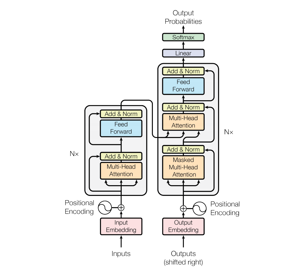
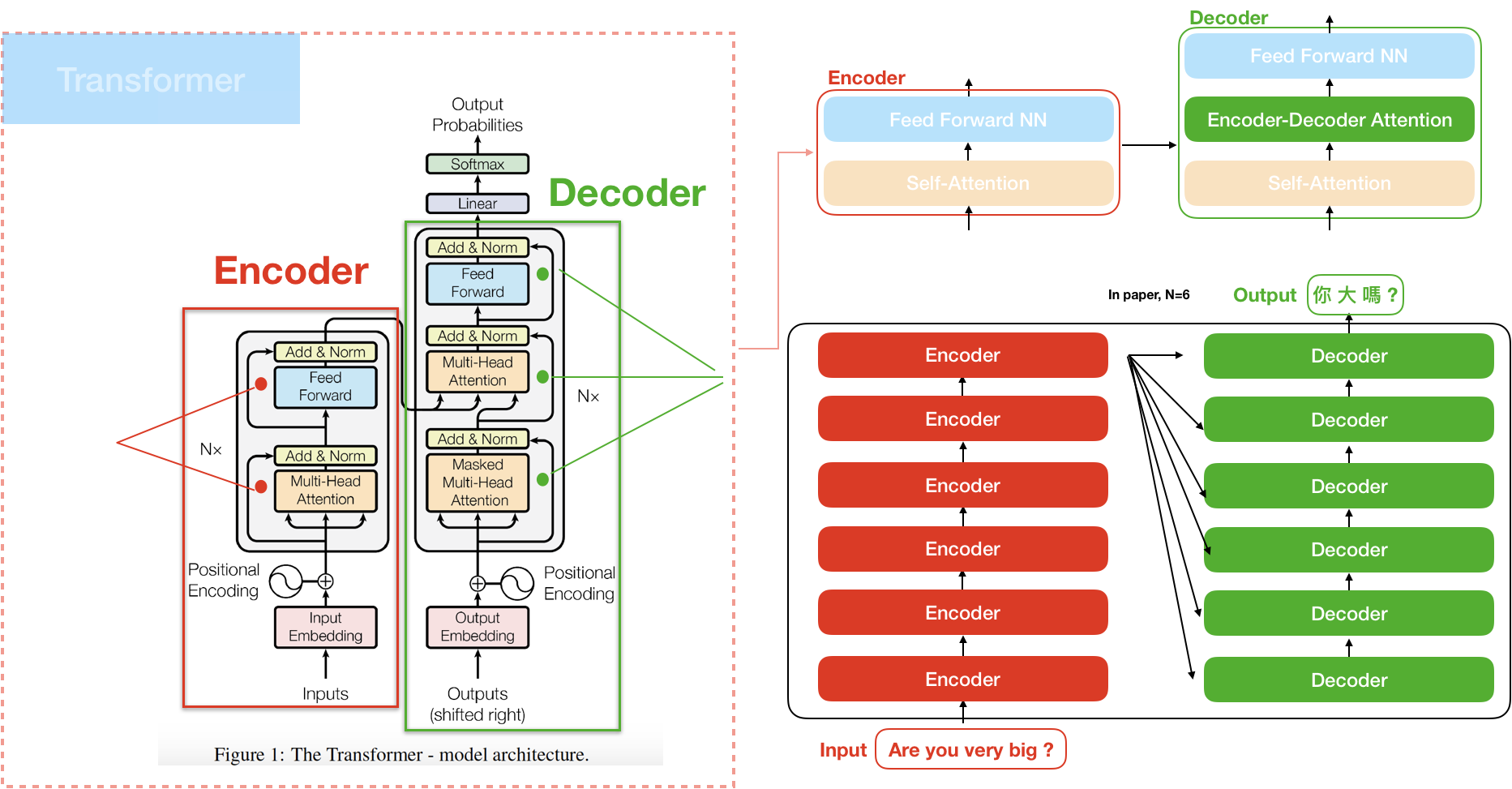
         return F.log_softmax(self.proj(x), dim=-1)

 # The Transformer follows this overall architecture using stacked self-attention and point-wise, fully connected layers for both the encoder and decoder, shown in the left and right halves of Figure 1, respectively.

 # ## Encoder and Decoder Stacks
 # ### Encoder
 # The encoder is composed of a stack of $N=6$ identical layers.
 def clones(module, N):
     "Produce N identical layers."
     return nn.ModuleList([copy.deepcopy(module) for _ in range(N)])

 class Encoder(nn.Module):
     "Core encoder is a stack of N layers"

     def __init__(self, layer, N):
         super(Encoder, self).__init__()
         self.layers = clones(layer, N)
         self.norm = LayerNorm(layer.size)

     def forward(self, x, mask):
         "Pass the input (and mask) through each layer in turn."
         for layer in self.layers:
             x = layer(x, mask)
         return self.norm(x)

 #layer normalization [(cite)](https://arxiv.org/abs/1607.06450). do on
 class LayerNorm(nn.Module):
     "Construct a layernorm module (See citation for details)."
     def __init__(self, features, eps=1e-6):
         super(LayerNorm, self).__init__()
         self.a_2 = nn.Parameter(torch.ones(features))
         self.b_2 = nn.Parameter(torch.zeros(features))
         self.eps = eps

     def forward(self, x):
         mean = x.mean(-1, keepdim=True)
         std = x.std(-1, keepdim=True)
         return self.a_2 * (x - mean) / (std + self.eps) + self.b_2

 # That is, the output of each sub-layer is $\mathrm{LayerNorm}(x + \mathrm{Sublayer}(x))$, where $\mathrm{Sublayer}(x)$ is the function implemented by the sub-layer itself.  We apply dropout [(cite)](http://jmlr.org/papers/v15/srivastava14a.html) to the output of each sub-layer, before it is added to the sub-layer input and normalized.
 # To facilitate these residual connections, all sub-layers in the model, as well as the embedding layers, produce outputs of dimension $d_{\text{model}}=512$.
 class SublayerConnection(nn.Module):
     """
     A residual connection followed by a layer norm.
     Note for code simplicity the norm is first as opposed to last.
     """

     def __init__(self, size, dropout):
         super(SublayerConnection, self).__init__()
         self.norm = LayerNorm(size)
         self.dropout = nn.Dropout(dropout)

     def forward(self, x, sublayer):
         "Apply residual connection to any sublayer with the same size."
         ret = x + self.dropout(sublayer(self.norm(x)))
         return ret

 # Each layer has two sub-layers. The first is a multi-head self-attention mechanism, and the second is a simple, position-wise fully connected feed-forward network.
 class EncoderLayer(nn.Module):
     "Encoder is made up of self-attn and feed forward (defined below)"

     def __init__(self, size, self_attn, feed_forward, dropout):
         super(EncoderLayer, self).__init__()
         self.self_attn = self_attn
         self.feed_forward = feed_forward
         self.sublayer = clones(SublayerConnection(size, dropout), 2)
         self.size = size

     def forward(self, x, mask):
         "Follow Figure 1 (left) for connections."
         x = self.sublayer[0](x, lambda x: self.self_attn(x, x, x, mask))
         # torch.Size([30, 10, 512])
         ret = self.sublayer[1](x, self.feed_forward)
         return ret

 # ### Decoder
 # The decoder is also composed of a stack of $N=6$ identical layers.
 class Decoder(nn.Module):
     "Generic N layer decoder with masking."

     def __init__(self, layer, N):
         super(Decoder, self).__init__()
         self.layers = clones(layer, N)
         self.norm = LayerNorm(layer.size)

     def forward(self, x, memory, src_mask, tgt_mask):
         for layer in self.layers:
             x = layer(x, memory, src_mask, tgt_mask)
         return self.norm(x)

 # In addition to the two sub-layers in each encoder layer, the decoder inserts a third sub-layer, which performs multi-head attention over the output of the encoder stack.  Similar to the encoder, we employ residual connections around each of the sub-layers, followed by layer normalization.
 class DecoderLayer(nn.Module):
     "Decoder is made of self-attn, src-attn, and feed forward (defined below)"

     def __init__(self, size, self_attn, src_attn, feed_forward, dropout):
         super(DecoderLayer, self).__init__()
         self.size = size
         self.self_attn = self_attn
         self.src_attn = src_attn
         self.feed_forward = feed_forward
         self.sublayer = clones(SublayerConnection(size, dropout), 3)

     def forward(self, x, memory, src_mask, tgt_mask):
         "Follow Figure 1 (right) for connections."
         m = memory
         x = self.sublayer[0](x, lambda x: self.self_attn(x, x, x, tgt_mask))
         x = self.sublayer[1](x, lambda x: self.src_attn(x, m, m, src_mask))
         return self.sublayer[2](x, self.feed_forward)

 # ### Attention
 # An attention function can be described as mapping a query and a set of key-value pairs to an output, where the query, keys, values, and output are all vectors.  The output is computed as a weighted sum of the values, where the weight assigned to each value is computed by a compatibility function of the query with the corresponding key.
 # We call our particular attention "Scaled Dot-Product Attention".   The input consists of queries and keys of dimension $d_k$, and values of dimension $d_v$.  We compute the dot products of the query with all keys, divide each by $\sqrt{d_k}$, and apply a softmax function to obtain the weights on the values.
 def attention(query, key, value, mask=None, dropout=None):
     "Compute 'Scaled Dot Product Attention'"
     # query,key,value:torch.Size([30, 8, 10, 64])
     # decoder mask:torch.Size([30, 1, 9, 9])
     d_k = query.size(-1)
     key_ = key.transpose(-2, -1)  # torch.Size([30, 8, 64, 10])
     # torch.Size([30, 8, 10, 10])
     scores = torch.matmul(query, key_) / math.sqrt(d_k)
     if mask is not None:
         # decoder scores:torch.Size([30, 8, 9, 9]),
         scores = scores.masked_fill(mask == 0, -1e9)
     p_attn = F.softmax(scores, dim=-1)
     if dropout is not None:
         p_attn = dropout(p_attn)
     return torch.matmul(p_attn, value), p_attn

 class MultiHeadedAttention(nn.Module):
     def __init__(self, h, d_model, dropout=0.1):
         "Take in model size and number of heads."
         super(MultiHeadedAttention, self).__init__()
         assert d_model % h == 0
         # We assume d_v always equals d_k
         self.d_k = d_model // h  # 64=512//8
         self.h = h
         self.linears = clones(nn.Linear(d_model, d_model), 4)
         self.attn = None
         self.dropout = nn.Dropout(p=dropout)

     def forward(self, query, key, value, mask=None):
         # query,key,value:torch.Size([30, 10, 512])
         if mask is not None:
             # Same mask applied to all h heads.
             mask = mask.unsqueeze(1)
         nbatches = query.size(0)
         # 1) Do all the linear projections in batch from d_model => h x d_k
         query, key, value = [l(x).view(nbatches, -1, self.h, self.d_k).transpose(1, 2)
                 for l, x in zip(self.linears, (query, key, value))]  # query,key,value:torch.Size([30, 8, 10, 64])
         # 2) Apply attention on all the projected vectors in batch.
         x, self.attn = attention(query, key, value, mask=mask,
                                  dropout=self.dropout)
         # 3) "Concat" using a view and apply a final linear.
         x = x.transpose(1, 2).contiguous().view(
             nbatches, -1, self.h * self.d_k)
         ret = self.linears[-1](x)  # torch.Size([30, 10, 512])
         return ret

 # ### Applications of Attention in our Model
 # The Transformer uses multi-head attention in three different ways:
 # 1) In "encoder-decoder attention" layers, the queries come from the previous decoder layer, and the memory keys and values come from the output of the encoder.   This allows every position in the decoder to attend over all positions in the input sequence.  This mimics the typical encoder-decoder attention mechanisms in sequence-to-sequence models such as [(cite)](https://arxiv.org/abs/1609.08144).
 # 2) The encoder contains self-attention layers.  In a self-attention layer all of the keys, values and queries come from the same place, in this case, the output of the previous layer in the encoder.   Each position in the encoder can attend to all positions in the previous layer of the encoder.
 # 3) Similarly, self-attention layers in the decoder allow each position in the decoder to attend to all positions in the decoder up to and including that position.  We need to prevent leftward information flow in the decoder to preserve the auto-regressive property.  We implement this inside of scaled dot-product attention by masking out (setting to $-\infty$) all values in the input of the softmax which correspond to illegal connections.
 # ## Position-wise Feed-Forward Networks
 class PositionwiseFeedForward(nn.Module):
     "Implements FFN equation."

     def __init__(self, d_model, d_ff, dropout=0.1):
         super(PositionwiseFeedForward, self).__init__()
         self.w_1 = nn.Linear(d_model, d_ff)
         self.w_2 = nn.Linear(d_ff, d_model)
         self.dropout = nn.Dropout(dropout)

     def forward(self, x):
         return self.w_2(self.dropout(F.relu(self.w_1(x))))

 # ## Embeddings and Softmax
 # Similarly to other sequence transduction models, we use learned embeddings to convert the input tokens and output tokens to vectors of dimension $d_{\text{model}}$.  We also use the usual learned linear transformation and softmax function to convert the decoder output to predicted next-token probabilities.  In our model, we share the same weight matrix between the two embedding layers and the pre-softmax linear transformation, similar to [(cite)](https://arxiv.org/abs/1608.05859). In the embedding layers, we multiply those weights by $\sqrt{d_{\text{model}}}$.
 class Embeddings(nn.Module):
     def __init__(self, d_model, vocab):
         super(Embeddings, self).__init__()
         self.lut = nn.Embedding(vocab, d_model)  # Embedding(11, 512)
         self.d_model = d_model

     def forward(self, x):
         return self.lut(x) * math.sqrt(self.d_model)

 # ## Positional Encoding
 class PositionalEncoding(nn.Module):
     "Implement the PE function."

     def __init__(self, d_model, dropout, max_len=5000):
         super(PositionalEncoding, self).__init__()
         self.dropout = nn.Dropout(p=dropout)

         # Compute the positional encodings once in log space.
         pe = torch.zeros(max_len, d_model)
         position = torch.arange(0., max_len).unsqueeze(1)
         div_term = torch.exp(torch.arange(0., d_model, 2)
                              * -(math.log(10000.0) / d_model))

         pe[:, 0::2] = torch.sin(position * div_term)
         pe[:, 1::2] = torch.cos(position * div_term)
         pe = pe.unsqueeze(0)
         self.register_buffer('pe', pe)

     def forward(self, x):
         x = x + Variable(self.pe[:, :x.size(1)],
                          requires_grad=False)
         return self.dropout(x)

 # We also experimented with using learned positional embeddings [(cite)](https://arxiv.org/pdf/1705.03122.pdf) instead, and found that the two versions produced nearly identical results.  We chose the sinusoidal version because it may allow the model to extrapolate to sequence lengths longer than the ones encountered during training.
 # ## Full Model
 def make_model(src_vocab, tgt_vocab, N=6,
                d_model=512, d_ff=2048, h=8, dropout=0.1):
     "Helper: Construct a model from hyperparameters."
     c = copy.deepcopy
     attn = MultiHeadedAttention(h, d_model)
     ff = PositionwiseFeedForward(d_model, d_ff, dropout)
     position = PositionalEncoding(d_model, dropout)
     model = EncoderDecoder(
         Encoder(EncoderLayer(d_model, c(attn), c(ff), dropout), N),
         Decoder(DecoderLayer(d_model, c(attn), c(attn),
                              c(ff), dropout), N),
         nn.Sequential(Embeddings(d_model, src_vocab), c(position)),
         nn.Sequential(Embeddings(d_model, tgt_vocab), c(position)),
         Generator(d_model, tgt_vocab))

     # This was important from their code.
     # Initialize parameters with Glorot / fan_avg.
     for p in model.parameters():
         if p.dim() > 1:
             nn.init.xavier_uniform_(p)
     return model

 # We also modify the self-attention sub-layer in the decoder stack to prevent positions from attending to subsequent positions.  This masking, combined with fact that the output embeddings are offset by one position, ensures that the predictions for position $i$ can depend only on the known outputs at positions less than $i$.

 def subsequent_mask(size):
     "Mask out subsequent positions when decoding."
     attn_shape = (1, size, size)
     subsequent_mask = np.triu(np.ones(attn_shape), k=1).astype('uint8')
     return torch.from_numpy(subsequent_mask) == 0

 # # Training
 # This section describes the training regime for our models.
 # > We stop for a quick interlude to introduce some of the tools
 # needed to train a standard encoder decoder model. First we define a batch object that holds the src and target sentences for training, as well as constructing the masks.
 # ## Batches and Masking

 class Batch:
     "Object for holding a batch of data with mask during training."

     def __init__(self, src, trg=None, pad=0):
         self.src = src
         self.src_mask = (src != pad).unsqueeze(-2)
         if trg is not None:
             self.trg = trg[:, :-1]
             self.trg_y = trg[:, 1:]
             self.trg_mask = self.make_std_mask(self.trg, pad)
             self.ntokens = (self.trg_y != pad).data.sum()

     @staticmethod
     def make_std_mask(tgt, pad):
         "Create a mask to hide padding and future words."
         tgt_mask = (tgt != pad).unsqueeze(-2)
         tgt_mask = tgt_mask & Variable(
             subsequent_mask(tgt.size(-1)).type_as(tgt_mask.data))
         return tgt_mask

 # Next we create a generic training and scoring function to keep track of loss. We pass in a generic loss compute function that also handles parameter updates.
 def run_epoch(data_iter, model, loss_compute):
     "Standard Training and Logging Function"
     start = time.time()
     total_tokens = 0
     total_loss = 0
     tokens = 0
     for i, batch in enumerate(data_iter):
         out = model.forward(batch.src, batch.trg,
                             batch.src_mask, batch.trg_mask)#torch.Size([30, 10]),torch.Size([30, 9]),torch.Size([30, 1, 10]),torch.Size([30, 9, 9])

         loss = loss_compute(out, batch.trg_y, batch.ntokens)
         total_loss += loss
         total_tokens += batch.ntokens
         tokens += batch.ntokens
         if i % 50 == 1:
             elapsed = time.time() - start
             print("Step: %d Loss: %f" %
                     (i, loss / batch.ntokens))
             start = time.time()
             tokens = 0

     return total_loss / total_tokens

 # ## Optimizer
 class NoamOpt:
     "Optim wrapper that implements rate."
     def __init__(self, model_size, factor, warmup, optimizer):
         self.optimizer = optimizer
         self._step = 0
         self.warmup = warmup
         self.factor = factor
         self.model_size = model_size
         self._rate = 0

     def step(self):
         "Update parameters and rate"
         self._step += 1
         rate = self.rate()
         for p in self.optimizer.param_groups:
             p['lr'] = rate
         self._rate = rate
         self.optimizer.step()

     def rate(self, step = None):
         "Implement `lrate` above"
         if step is None:
             step = self._step
         return self.factor *(self.model_size ** (-0.5) *min(step ** (-0.5), step * self.warmup ** (-1.5)))

 def get_std_opt(model):
     return NoamOpt(model.src_embed[0].d_model, 2, 4000,
             torch.optim.Adam(model.parameters(), lr=0, betas=(0.9, 0.98), eps=1e-9))
 # Three settings of the lrate hyperparameters.
 opts = [NoamOpt(512, 1, 4000, None),
         NoamOpt(512, 1, 8000, None),
         NoamOpt(256, 1, 4000, None)]

 # ## Regularization
 # ### Label Smoothing
 # During training, we employed label smoothing . This hurts perplexity, as the model learns to be more unsure, but improves accuracy and BLEU score.
 class LabelSmoothing(nn.Module):
     "Implement label smoothing."
     def __init__(self, size, padding_idx, smoothing=0.0):
         super(LabelSmoothing, self).__init__()
         self.criterion = nn.KLDivLoss(size_average=False)
         self.padding_idx = padding_idx
         self.confidence = 1.0 - smoothing
         self.smoothing = smoothing
         self.size = size
         self.true_dist = None

     def forward(self, x, target):
         assert x.size(1) == self.size
         true_dist = x.data.clone()
         true_dist.fill_(self.smoothing / (self.size - 2))
         true_dist.scatter_(1, target.data.unsqueeze(1), self.confidence)
         true_dist[:, self.padding_idx] = 0
         mask = torch.nonzero(target.data == self.padding_idx)
         if mask.dim() > 0:
             true_dist.index_fill_(0, mask.squeeze(), 0.0)
         self.true_dist = true_dist
         return self.criterion(x, Variable(true_dist, requires_grad=False))

 # > Here we can see an example of how the mass is distributed to the words based on confidence.
 # crit = LabelSmoothing(5, 0, 0.4)
 # predict = torch.FloatTensor([[0, 0.2, 0.7, 0.1, 0],
 #                              [0, 0.2, 0.7, 0.1, 0],
 #                              [0, 0.2, 0.7, 0.1, 0]])
 # v = crit(Variable(predict.log()),
 #          Variable(torch.LongTensor([2, 1, 0])))

 # crit = LabelSmoothing(5, 0, 0.1)
 # def loss(x):
 #     d = x + 3 * 1
 #     predict = torch.FloatTensor([[0, x / d, 1 / d, 1 / d, 1 / d],
 #                                  ])
 #     # print(predict)
 #     return crit(Variable(predict.log()),
 #                  Variable(torch.LongTensor([1]))).item()

 # # A First  Example
 # > We can begin by trying out a simple copy-task. Given a random set of input symbols from a small vocabulary, the goal is to generate back those same symbols.
 # ## Synthetic Data
 def data_gen(V, batch, nbatches):
     "Generate random data for a src-tgt copy task."
     for i in range(nbatches):
         data = torch.from_numpy(np.random.randint(1, V, size=(batch, 10)))#torch.Size([30, 10])
         data[:, 0] = 1 #start
         src = Variable(data, requires_grad=False)
         tgt = Variable(data, requires_grad=False)
         yield Batch(src, tgt, 0)
 # data_gen(11,30,20)

 # ## Loss Computation
 class SimpleLossCompute:
     "A simple loss compute and train function."
     def __init__(self, generator, criterion, opt=None):
         self.generator = generator
         self.criterion = criterion
         self.opt = opt

     def __call__(self, x, y, norm):
         x = self.generator(x)
         loss = self.criterion(x.contiguous().view(-1, x.size(-1)),
                               y.contiguous().view(-1)) / norm
         loss.backward()
         if self.opt is not None:
             self.opt.step()
             self.opt.optimizer.zero_grad()
         return loss.item() * norm

 # ## Greedy Decoding
 # Train the simple copy task.
 V = 11
 criterion = LabelSmoothing(size=V, padding_idx=0, smoothing=0.0)
 model = make_model(V, V, N=2)
 model_opt = NoamOpt(model.src_embed[0].d_model, 1, 400,
         torch.optim.Adam(model.parameters(), lr=0.01, betas=(0.9, 0.98), eps=1e-9))

 for epoch in range(5):
     model.train()
     run_epoch(data_gen(V, 30, 20), model,
               SimpleLossCompute(model.generator, criterion, model_opt))
     model.eval()
     print(run_epoch(data_gen(V, 30, 5), model,
                     SimpleLossCompute(model.generator, criterion, None)))

 #This code predicts a translation using greedy decoding for simplicity.
 def greedy_decode(model, src, src_mask, max_len, start_symbol):
     memory = model.encode(src, src_mask)
     ys = torch.ones(1, 1).fill_(start_symbol).type_as(src.data)#fill start symbol
     for i in range(max_len-1):
         out = model.decode(memory, src_mask,
                            Variable(ys),
                            Variable(subsequent_mask(ys.size(1))
                                     .type_as(src.data)))
         prob = model.generator(out[:, -1])
         _, next_word = torch.max(prob, dim = 1)
         next_word = next_word.data[0]
         ys = torch.cat([ys,
                         torch.ones(1, 1).type_as(src.data).fill_(next_word)], dim=1)
     return ys

 model.eval()
 src = Variable(torch.LongTensor([[1,2,3,4,5,6,7,8,9,10]]) )
 src_mask = Variable(torch.ones(1, 1, 10) )
 print(greedy_decode(model, src, src_mask, max_len=10, start_symbol=1))

 '''
 # # A Real World Example
 #
 # > Now we consider a real-world example using the IWSLT German-English Translation task. This task is much smaller than the WMT task considered in the paper, but it illustrates the whole system. We also show how to use multi-gpu processing to make it really fast.

 #!pip install torchtext spacy
 #!python -m spacy download en
 #!python -m spacy download de

 # ## Training Data and Batching
 global max_src_in_batch, max_tgt_in_batch
 def batch_size_fn(new, count, sofar):
     "Keep augmenting batch and calculate total number of tokens + padding."
     global max_src_in_batch, max_tgt_in_batch
     if count == 1:
         max_src_in_batch = 0
         max_tgt_in_batch = 0
     max_src_in_batch = max(max_src_in_batch,  len(new.src))
     max_tgt_in_batch = max(max_tgt_in_batch,  len(new.trg) + 2)
     src_elements = count * max_src_in_batch
     tgt_elements = count * max_tgt_in_batch

     return max(src_elements, tgt_elements)

 # ## Data Loading
 # > We will load the dataset using torchtext and spacy for tokenization. 

 # For data loading.
 from torchtext import data, datasets

 if True:
     import spacy
     spacy_de = spacy.load('de')
     spacy_en = spacy.load('en')

     def tokenize_de(text):
         return [tok.text for tok in spacy_de.tokenizer(text)]

     def tokenize_en(text):
         return [tok.text for tok in spacy_en.tokenizer(text)]

     BOS_WORD = '<s>'
     EOS_WORD = '</s>'
     BLANK_WORD = "<blank>"
     SRC = data.Field(tokenize=tokenize_de, pad_token=BLANK_WORD)
     TGT = data.Field(tokenize=tokenize_en, init_token = BOS_WORD,
                      eos_token = EOS_WORD, pad_token=BLANK_WORD)

     MAX_LEN = 100
     train, val, test = datasets.IWSLT.splits(
         exts=('.de', '.en'), fields=(SRC, TGT),
         filter_pred=lambda x: len(vars(x)['src']) <= MAX_LEN and
             len(vars(x)['trg']) <= MAX_LEN)
     MIN_FREQ = 2
     SRC.build_vocab(train.src, min_freq=MIN_FREQ)
     TGT.build_vocab(train.trg, min_freq=MIN_FREQ)

 # > Batching matters a ton for speed. We want to have very evenly divided batches, with absolutely minimal padding. To do this we have to hack a bit around the default torchtext batching. This code patches their default batching to make sure we search over enough sentences to find tight batches.
 # ## Iterators

 class MyIterator(data.Iterator):
     def create_batches(self):
         if self.train:
             def pool(d, random_shuffler):
                 for p in data.batch(d, self.batch_size * 100):
                     p_batch = data.batch(
                         sorted(p, key=self.sort_key),
                         self.batch_size, self.batch_size_fn)
                     for b in random_shuffler(list(p_batch)):
                         yield b
             self.batches = pool(self.data(), self.random_shuffler)

         else:
             self.batches = []
             for b in data.batch(self.data(), self.batch_size,
                                           self.batch_size_fn):
                 self.batches.append(sorted(b, key=self.sort_key))

 def rebatch(pad_idx, batch):
     "Fix order in torchtext to match ours"
     src, trg = batch.src.transpose(0, 1), batch.trg.transpose(0, 1)
     return Batch(src, trg, pad_idx)

 # ## Multi-GPU Training
 # > Finally to really target fast training, we will use multi-gpu. This code implements multi-gpu word generation. It is not specific to transformer so I won't go into too much detail. The idea is to split up word generation at training time into chunks to be processed in parallel across many different gpus. We do this using pytorch parallel primitives:
 #
 # * replicate - split modules onto different gpus.
 # * scatter - split batches onto different gpus
 # * parallel_apply - apply module to batches on different gpus
 # * gather - pull scattered data back onto one gpu.
 # * nn.DataParallel - a special module wrapper that calls these all before evaluating.
 # 

 # Skip if not interested in multigpu.
 class MultiGPULossCompute:
     "A multi-gpu loss compute and train function."
     def __init__(self, generator, criterion, devices, opt=None, chunk_size=5):
         # Send out to different gpus.
         self.generator = generator
         self.criterion = nn.parallel.replicate(criterion,
                                                devices=devices)
         self.opt = opt
         self.devices = devices
         self.chunk_size = chunk_size

     def __call__(self, out, targets, normalize):
         total = 0.0
         generator = nn.parallel.replicate(self.generator,
                                                 devices=self.devices)
         out_scatter = nn.parallel.scatter(out,
                                           target_gpus=self.devices)
         out_grad = [[] for _ in out_scatter]
         targets = nn.parallel.scatter(targets,
                                       target_gpus=self.devices)

         # Divide generating into chunks.
         chunk_size = self.chunk_size
         for i in range(0, out_scatter[0].size(1), chunk_size):
             # Predict distributions
             out_column = [[Variable(o[:, i:i+chunk_size].data,
                                     requires_grad=self.opt is not None)]
                            for o in out_scatter]
             gen = nn.parallel.parallel_apply(generator, out_column)

             # Compute loss.
             y = [(g.contiguous().view(-1, g.size(-1)),
                   t[:, i:i+chunk_size].contiguous().view(-1))
                  for g, t in zip(gen, targets)]
             loss = nn.parallel.parallel_apply(self.criterion, y)

             # Sum and normalize loss
             l = nn.parallel.gather(loss,
                                    target_device=self.devices[0])
             l = l.sum()[0] / normalize
             total += l.data[0]

             # Backprop loss to output of transformer
             if self.opt is not None:
                 l.backward()
                 for j, l in enumerate(loss):
                     out_grad[j].append(out_column[j][0].grad.data.clone())

         # Backprop all loss through transformer.
         if self.opt is not None:
             out_grad = [Variable(torch.cat(og, dim=1)) for og in out_grad]
             o1 = out
             o2 = nn.parallel.gather(out_grad,
                                     target_device=self.devices[0])
             o1.backward(gradient=o2)
             self.opt.step()
             self.opt.optimizer.zero_grad()
         return total * normalize

 # > Now we create our model, criterion, optimizer, data iterators, and paralelization
 # GPUs to use
 devices = [0, 1, 2, 3]
 if True:
     pad_idx = TGT.vocab.stoi["<blank>"]
     model = make_model(len(SRC.vocab), len(TGT.vocab), N=6)
     model.cuda()
     criterion = LabelSmoothing(size=len(TGT.vocab), padding_idx=pad_idx, smoothing=0.1)
     criterion.cuda()
     BATCH_SIZE = 12000
     train_iter = MyIterator(train, batch_size=BATCH_SIZE, device=0,
                             repeat=False, sort_key=lambda x: (len(x.src), len(x.trg)),
                             batch_size_fn=batch_size_fn, train=True)
     valid_iter = MyIterator(val, batch_size=BATCH_SIZE, device=0,
                             repeat=False, sort_key=lambda x: (len(x.src), len(x.trg)),
                             batch_size_fn=batch_size_fn, train=False)
     model_par = nn.DataParallel(model, device_ids=devices)
 None

 # > Now we train the model. I will play with the warmup steps a bit, but everything else uses the default parameters.  On an AWS p3.8xlarge with 4 Tesla V100s, this runs at ~27,000 tokens per second with a batch size of 12,000
 # ## Training the System
 #!wget https://s3.amazonaws.com/opennmt-models/iwslt.pt

 if False:
     model_opt = NoamOpt(model.src_embed[0].d_model, 1, 2000,
             torch.optim.Adam(model.parameters(), lr=0, betas=(0.9, 0.98), eps=1e-9))
     for epoch in range(10):
         model_par.train()
         run_epoch((rebatch(pad_idx, b) for b in train_iter),
                   model_par,
                   MultiGPULossCompute(model.generator, criterion,
                                       devices=devices, opt=model_opt))
         model_par.eval()
         loss = run_epoch((rebatch(pad_idx, b) for b in valid_iter),
                           model_par,
                           MultiGPULossCompute(model.generator, criterion,
                           devices=devices, opt=None))
         print(loss)
 else:
     model = torch.load("iwslt.pt")

 # > Once trained we can decode the model to produce a set of translations. Here we simply translate the first sentence in the validation set. This dataset is pretty small so the translations with greedy search are reasonably accurate. 

 for i, batch in enumerate(valid_iter):
     src = batch.src.transpose(0, 1)[:1]
     src_mask = (src != SRC.vocab.stoi["<blank>"]).unsqueeze(-2)
     out = greedy_decode(model, src, src_mask,
                         max_len=60, start_symbol=TGT.vocab.stoi["<s>"])
     print("Translation:", end="\t")
     for i in range(1, out.size(1)):
         sym = TGT.vocab.itos[out[0, i]]
         if sym == "</s>": break
         print(sym, end =" ")
     print()
     print("Target:", end="\t")
     for i in range(1, batch.trg.size(0)):
         sym = TGT.vocab.itos[batch.trg.data[i, 0]]
         if sym == "</s>": break
         print(sym, end =" ")
     print()
     break

 # # Additional Components: BPE, Search, Averaging

 # > So this mostly covers the transformer model itself. There are four aspects that we didn't cover explicitly. We also have all these additional features implemented in [OpenNMT-py](https://github.com/opennmt/opennmt-py).
 #
 # 

 # > 1) BPE/ Word-piece: We can use a library to first preprocess the data into subword units. See Rico Sennrich's [subword-nmt](https://github.com/rsennrich/subword-nmt) implementation. These models will transform the training data to look like this:
 # ▁Die ▁Protokoll datei ▁kann ▁ heimlich ▁per ▁E - Mail ▁oder ▁FTP ▁an ▁einen ▁bestimmte n ▁Empfänger ▁gesendet ▁werden .
 # > 2) Shared Embeddings: When using BPE with shared vocabulary we can share the same weight vectors between the source / target / generator. See the [(cite)](https://arxiv.org/abs/1608.05859) for details. To add this to the model simply do this:

 if False:
     model.src_embed[0].lut.weight = model.tgt_embeddings[0].lut.weight
     model.generator.lut.weight = model.tgt_embed[0].lut.weight

 # > 3) Beam Search: This is a bit too complicated to cover here. See the [OpenNMT-py](https://github.com/OpenNMT/OpenNMT-py/blob/master/onmt/translate/Beam.py) for a pytorch implementation.
 # > 4) Model Averaging: The paper averages the last k checkpoints to create an ensembling effect. We can do this after the fact if we have a bunch of models:

 def average(model, models):
     "Average models into model"
     for ps in zip(*[m.params() for m in [model] + models]):
         p[0].copy_(torch.sum(*ps[1:]) / len(ps[1:]))

 # # Results
 #
 # On the WMT 2014 English-to-German translation task, the big transformer model (Transformer (big)
 # in Table 2) outperforms the best previously reported models (including ensembles) by more than 2.0
 # BLEU, establishing a new state-of-the-art BLEU score of 28.4. The configuration of this model is
 # listed in the bottom line of Table 3. Training took 3.5 days on 8 P100 GPUs. Even our base model
 # surpasses all previously published models and ensembles, at a fraction of the training cost of any of
 # the competitive models.
 #
 # On the WMT 2014 English-to-French translation task, our big model achieves a BLEU score of 41.0,
 # outperforming all of the previously published single models, at less than 1/4 the training cost of the
 # previous state-of-the-art model. The Transformer (big) model trained for English-to-French used
 # dropout rate Pdrop = 0.1, instead of 0.3.
 #
 # 

 # > The code we have written here is a version of the base model. There are fully trained version of this system available here  [(Example Models)](http://opennmt.net/Models-py/).
 # >
 # > With the addtional extensions in the last section, the OpenNMT-py replication gets to 26.9 on EN-DE WMT. Here I have loaded in those parameters to our reimplemenation. 

 get_ipython().system('wget https://s3.amazonaws.com/opennmt-models/en-de-model.pt')

 model, SRC, TGT = torch.load("en-de-model.pt")

 model.eval()
 sent = "▁The ▁log ▁file ▁can ▁be ▁sent ▁secret ly ▁with ▁email ▁or ▁FTP ▁to ▁a ▁specified ▁receiver".split()
 src = torch.LongTensor([[SRC.stoi[w] for w in sent]])
 src = Variable(src)
 src_mask = (src != SRC.stoi["<blank>"]).unsqueeze(-2)
 out = greedy_decode(model, src, src_mask,
                     max_len=60, start_symbol=TGT.stoi["<s>"])
 print("Translation:", end="\t")
 trans = "<s> "
 for i in range(1, out.size(1)):
     sym = TGT.itos[out[0, i]]
     if sym == "</s>": break
     trans += sym + " "
 print(trans)

 # ## Attention Visualization
 #
 # > Even with a greedy decoder the translation looks pretty good. We can further visualize it to see what is happening at each layer of the attention 

 tgt_sent = trans.split()
 def draw(data, x, y, ax):
     seaborn.heatmap(data,
                     xticklabels=x, square=True, yticklabels=y, vmin=0.0, vmax=1.0,
                     cbar=False, ax=ax)

 for layer in range(1, 6, 2):
     fig, axs = plt.subplots(1,4, figsize=(20, 10))
     print("Encoder Layer", layer+1)
     for h in range(4):
         draw(model.encoder.layers[layer].self_attn.attn[0, h].data,
             sent, sent if h ==0 else [], ax=axs[h])
     plt.show()

 for layer in range(1, 6, 2):
     fig, axs = plt.subplots(1,4, figsize=(20, 10))
     print("Decoder Self Layer", layer+1)
     for h in range(4):
         draw(model.decoder.layers[layer].self_attn.attn[0, h].data[:len(tgt_sent), :len(tgt_sent)],
             tgt_sent, tgt_sent if h ==0 else [], ax=axs[h])
     plt.show()
     print("Decoder Src Layer", layer+1)
     fig, axs = plt.subplots(1,4, figsize=(20, 10))
     for h in range(4):
         draw(model.decoder.layers[layer].self_attn.attn[0, h].data[:len(tgt_sent), :len(sent)],
             sent, tgt_sent if h ==0 else [], ax=axs[h])
     plt.show()

 '''