Deep Learning 学习随记（六）Linear Decoder 线性解码

线性解码器（Linear Decoder）

前面第一章提到稀疏自编码器（http://www.cnblogs.com/bzjia-blog/p/SparseAutoencoder.html）的三层网络结构，我们要满足最后一层的输出：a^（3）≈a^（1）（即输入值x）的近似重建。考虑到在最后一层的a^（3）=f（z^（3）），这里f一般用sigmoid函数或tanh函数等非线性函数，而将输出界定在一个范围内（比如sigmoid函数使结果在[0，1]中）。这对于有些数据组，例如MNIST手写数字库中其输入输出范围符合极佳，但并不是所有的情况都满足这个条件。例如，若采用PCA白化，输入将不再限制于[0,1]，虽可通过缩放数据来确保其符合特定范围内，但显然，这不是最好的方式。

因此，这里提到的Linear Decoder就是通过在最后一层用激励函数：a^（3） = z^（3）（也即f（z）=z）来实现。这里要注意到，只是在最后一层用这个激励函数，其他隐层的激励函数仍然是sigmoid函数或者tanh函数，我们仅在输出层中使用线性激励机制。

这样一来，在求梯度的时候，公式：

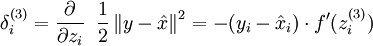
就应该改成：

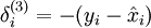
这个是显然的，因为f'（z）=1。其他层的都不需要改变。

练习：

这里讲义给出了一个练习，基本跟稀疏自编码一样，只有几处需要稍微改动一下。

linearDecoderExercise.m

%% CS294A/CS294W Linear Decoder Exercise

%  Instructions
%  ------------
%
%  This file contains code that helps you get started on the
%  linear decoder exericse. For this exercise, you will only need to modify
%  the code in sparseAutoencoderLinearCost.m. You will not need to modify
%  any code in this file.

%%======================================================================
%% STEP : Initialization
%  Here we initialize some parameters used for the exercise.

imageChannels = ;     % number of channels (rgb, so )

patchDim   = ;          % patch dimension
numPatches = ;   % number of patches

visibleSize = patchDim * patchDim * imageChannels;  % number of input units
outputSize  = visibleSize;   % number of output units
hiddenSize  = ;           % number of hidden units 

sparsityParam = 0.035; % desired average activation of the hidden units.
lambda = 3e-;         % weight decay parameter
beta = ;              % weight of sparsity penalty term       

epsilon = 0.1;           % epsilon for ZCA whitening

%%======================================================================
%% STEP : Create and modify sparseAutoencoderLinearCost.m to use a linear decoder,
%          and check gradients
%  You should copy sparseAutoencoderCost.m from your earlier exercise
%  and rename it to sparseAutoencoderLinearCost.m.
%  Then you need to rename the function from sparseAutoencoderCost to
%  sparseAutoencoderLinearCost, and modify it so that the sparse autoencoder
%  uses a linear decoder instead. Once that is done, you should check
% your gradients to verify that they are correct.

% NOTE: Modify sparseAutoencoderCost first!

% To speed up gradient checking, we will use a reduced network and some
% dummy patches

debugHiddenSize = ;
debugvisibleSize = ;
patches = rand([ ]);
theta = initializeParameters(debugHiddenSize, debugvisibleSize); 

[cost, grad] = sparseAutoencoderLinearCost(theta, debugvisibleSize, debugHiddenSize, ...
                                           lambda, sparsityParam, beta, ...
                                           patches);

% Check gradients
numGrad = computeNumericalGradient( @(x) sparseAutoencoderLinearCost(x, debugvisibleSize, debugHiddenSize, ...
                                                  lambda, sparsityParam, beta, ...
                                                  patches), theta);

% Use this to visually compare the gradients side by side
disp([numGrad grad]); 

diff = norm(numGrad-grad)/norm(numGrad+grad);
% Should be small. In our implementation, these values are usually less than 1e-.
disp(diff); 

assert(diff < 1e-, 'Difference too large. Check your gradient computation again');

% NOTE: Once your gradients check out, you should run step  again to
%       reinitialize the parameters
%}

%%======================================================================
%% STEP : Learn features on small patches
%  In this step, you will use your sparse autoencoder (which now uses a
%  linear decoder) to learn features on small patches sampled from related
%  images.

%% STEP 2a: Load patches
%  In this step, we load 100k patches sampled from the STL10 dataset and
%  visualize them. Note that these patches have been scaled to [,]

load stlSampledPatches.mat

displayColorNetwork(patches(:, :));

%% STEP 2b: Apply preprocessing
%  In this sub-step, we preprocess the sampled patches, in particular,
%  ZCA whitening them.
%
%  In a later exercise on convolution and pooling, you will need to replicate
%  exactly the preprocessing steps you apply to these patches before
%  using the autoencoder to learn features on them. Hence, we will save the
%  ZCA whitening and mean image matrices together with the learned features
%  later on.

% Subtract mean patch (hence zeroing the mean of the patches)
meanPatch = mean(patches, );
patches = bsxfun(@minus, patches, meanPatch);

% Apply ZCA whitening
sigma = patches * patches' / numPatches;
[u, s, v] = svd(sigma);
ZCAWhite = u * diag( ./ sqrt(diag(s) + epsilon)) * u';
patches = ZCAWhite * patches;

displayColorNetwork(patches(:, :));

%% STEP 2c: Learn features
%  You will now use your sparse autoencoder (with linear decoder) to learn
%  features on the preprocessed patches. This should take around  minutes.

theta = initializeParameters(hiddenSize, visibleSize);

% Use minFunc to minimize the function
addpath minFunc/

options = struct;
options.Method = 'lbfgs';
options.maxIter = ;
options.display = 'on';

[optTheta, cost] = minFunc( @(p) sparseAutoencoderLinearCost(p, ...
                                   visibleSize, hiddenSize, ...
                                   lambda, sparsityParam, ...
                                   beta, patches), ...
                              theta, options);

% Save the learned features and the preprocessing matrices for use in
% the later exercise on convolution and pooling
fprintf('Saving learned features and preprocessing matrices...\n');
save('STL10Features.mat', 'optTheta', 'ZCAWhite', 'meanPatch');
fprintf('Saved\n');

%% STEP 2d: Visualize learned features

W = reshape(optTheta(:visibleSize * hiddenSize), hiddenSize, visibleSize);
b = optTheta(*hiddenSize*visibleSize+:*hiddenSize*visibleSize+hiddenSize);
displayColorNetwork( (W*ZCAWhite)');

 sparseAutoencoderLinearCost.m

function [cost,grad,features] = sparseAutoencoderLinearCost(theta, visibleSize, hiddenSize, ...
                                                            lambda, sparsityParam, beta, data)
% -------------------- YOUR CODE HERE --------------------
% Instructions:
%   Copy sparseAutoencoderCost in sparseAutoencoderCost.m from your
%   earlier exercise onto this file, renaming the function to
%   sparseAutoencoderLinearCost, and changing the autoencoder to use a
%   linear decoder.

% visibleSize: the number of input units (probably 64)
% hiddenSize: the number of hidden units (probably 25)
% lambda: weight decay parameter
% sparsityParam: The desired average activation for the hidden units (denoted in the lecture
%                           notes by the greek alphabet rho, which looks like a lower-case "p").
% beta: weight of sparsity penalty term
% data: Our 64x10000 matrix containing the training data.  So, data(:,i) is the i-th training example. 

% The input theta is a vector (because minFunc expects the parameters to be a vector).
% We first convert theta to the (W1, W2, b1, b2) matrix/vector format, so that this
% follows the notation convention of the lecture notes. 

%将长向量转换成每一层的权值矩阵和偏置向量值
W1 = reshape(theta(1:hiddenSize*visibleSize), hiddenSize, visibleSize);
W2 = reshape(theta(hiddenSize*visibleSize+1:2*hiddenSize*visibleSize), visibleSize, hiddenSize);
b1 = theta(2*hiddenSize*visibleSize+1:2*hiddenSize*visibleSize+hiddenSize);
b2 = theta(2*hiddenSize*visibleSize+hiddenSize+1:end);

% Cost and gradient variables (your code needs to compute these values).
% Here, we initialize them to zeros.
cost = 0;
W1grad = zeros(size(W1));
W2grad = zeros(size(W2));
b1grad = zeros(size(b1));
b2grad = zeros(size(b2));

%% ---------- YOUR CODE HERE --------------------------------------

Jcost = 0;%直接误差
Jweight = 0;%权值惩罚
Jsparse = 0;%稀疏性惩罚
[n m] = size(data);%m为样本的个数，n为样本的特征数

%前向算法计算各神经网络节点的线性组合值和active值
z2 = W1*data+repmat(b1,1,m);%注意这里一定要将b1向量复制扩展成m列的矩阵
a2 = sigmoid(z2);
z3 = W2*a2+repmat(b2,1,m);
a3 = z3;                                             %线性解码器************

% 计算预测产生的误差
Jcost = (0.5/m)*sum(sum((a3-data).^2));

%计算权值惩罚项
Jweight = (1/2)*(sum(sum(W1.^2))+sum(sum(W2.^2)));

%计算稀释性规则项
rho = (1/m).*sum(a2,2);%求出第一个隐含层的平均值向量
Jsparse = sum(sparsityParam.*log(sparsityParam./rho)+ ...
        (1-sparsityParam).*log((1-sparsityParam)./(1-rho)));

%损失函数的总表达式
cost = Jcost+lambda*Jweight+beta*Jsparse;

%反向算法求出每个节点的误差值
d3 = -(data-a3);                                         %线性解码器**************
sterm = beta*(-sparsityParam./rho+(1-sparsityParam)./(1-rho));%因为加入了稀疏规则项，所以
                                                             %计算偏导时需要引入该项
d2 = (W2'*d3+repmat(sterm,1,m)).*sigmoidInv(z2); 

%计算W1grad
W1grad = W1grad+d2*data';
W1grad = (1/m)*W1grad+lambda*W1;

%计算W2grad
W2grad = W2grad+d3*a2';
W2grad = (1/m).*W2grad+lambda*W2;

%计算b1grad
b1grad = b1grad+sum(d2,2);
b1grad = (1/m)*b1grad;%注意b的偏导是一个向量，所以这里应该把每一行的值累加起来

%计算b2grad
b2grad = b2grad+sum(d3,2);
b2grad = (1/m)*b2grad;

%-------------------------------------------------------------------
% After computing the cost and gradient, we will convert the gradients back
% to a vector format (suitable for minFunc).  Specifically, we will unroll
% your gradient matrices into a vector.

grad = [W1grad(:) ; W2grad(:) ; b1grad(:) ; b2grad(:)];

end

%-------------------------------------------------------------------
% Here's an implementation of the sigmoid function, which you may find useful
% in your computation of the costs and the gradients.  This inputs a (row or
% column) vector (say (z1, z2, z3)) and returns (f(z1), f(z2), f(z3)). 

function sigm = sigmoid(x)

    sigm = 1 ./ (1 + exp(-x));
end

%sigmoid函数的逆函数
function sigmInv = sigmoidInv(x)

    sigmInv = sigmoid(x).*(1-sigmoid(x));
end

只是对稀疏自编码器的代码进行了两处稍微的改动。

结果：

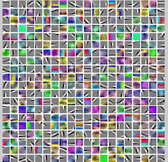
学习到的特征也放在了STL10Features.mat里，将要在下一章的练习中用到。

PS:讲义地址：

http://deeplearning.stanford.edu/wiki/index.php/Linear_Decoders

http://deeplearning.stanford.edu/wiki/index.php/Exercise:Learning_color_features_with_Sparse_Autoencoders