pandas时间序列学习笔记

目录

• 创建一个时间序列
  • pd.date_range()
  • info()
• asfred(）
• shifted（），滞后函数
• diff()求差分
  • 加减乘除
• DataFrame.reindex()
• 通过data_range指定时间序列的起止时间
• 通过as.fred()指定时间序列的间隔
• interpolate()
• resample()
• 补充一个绘图的参数
  • first（）
• pct_change()
  • pd.contact()
  • agg()
• rolling window functions.
• rolling()
• join()
• quantile()
  • append()
• pandas 中统计累计次数
  • .cumsum()
  • .cumprod()
  • np.prod这个是numpy里面求阶乘的
• 一个案例学习
• seed()
• random walk
• choice()
• Relationships between time series: correlation
• heatmap()
• Select index components & import data
• groupby()
• 最后一行or一列的表示方法
• sort_values
• plotz中的参数kind
• to_excel()

创建一个时间序列

pd.date_range()

这个函数是手动设置时间的范围，参数periods是设置时间间隔的

# Create the range of dates here
seven_days = pd.date_range('2017-1-1', periods=7)
# Iterate over the dates and print the number and name of the weekday
for day in seven_days:
    print(day.dayofweek, day.weekday_name)
<script.py> output:
    6 Sunday
    0 Monday
    1 Tuesday
    2 Wednesday
    3 Thursday
    4 Friday
    5 Saturday

info()

查看数据索引和内存信息的

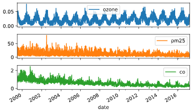
data = pd.read_csv('nyc.csv')
# Inspect data
print(data.info())
# Convert the date column to datetime64
data.date = pd.to_datetime(data.date)
# Set date column as index
data.set_index('date', inplace=True)
# Inspect data
print(data.info())
# Plot data
data.plot(subplots=True)
plt.show()
<script.py> output:
    <class 'pandas.core.frame.DataFrame'>
    RangeIndex: 6317 entries, 0 to 6316
    Data columns (total 4 columns):
    date     6317 non-null object
    ozone    6317 non-null float64
    pm25     6317 non-null float64
    co       6317 non-null float64
    dtypes: float64(3), object(1)
    memory usage: 197.5+ KB
    None
    <class 'pandas.core.frame.DataFrame'>
    DatetimeIndex: 6317 entries, 1999-07-01 to 2017-03-31
    Data columns (total 3 columns):
    ozone    6317 non-null float64
    pm25     6317 non-null float64
    co       6317 non-null float64
    dtypes: float64(3)
    memory usage: 197.4 KB
    None

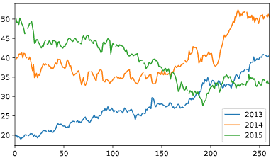
# Create dataframe prices here
prices = pd.DataFrame()
# Select data for each year and concatenate with prices here
for year in ['2013', '2014', '2015']:
    price_per_year = yahoo.loc[year, ['price']].reset_index(drop=True)
    price_per_year.rename(columns={'price': year}, inplace=True)
    prices = pd.concat([prices, price_per_year], axis=1)
# Plot prices
prices.plot()
plt.show()

asfred(）

给已经存在的时间序列调整时间间隔

# Inspect data
print(co.info())
# Set the frequency to calendar daily
co = co.asfreq('D')
# Plot the data
co.plot(subplots=True)
plt.show()
# Set frequency to monthly
co = co.asfreq('M')
# Plot the data
co.plot(subplots=True)
plt.show()

shifted（），滞后函数

等价于r里面的lag（）

peroid参数指定滞后阶数

\(x_t\)/\(x_{t-1}\)

diff()求差分

\(x_t\)-\(x_{t-1}\)

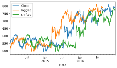
# Import data here
google = pd.read_csv('google.csv', parse_dates=['Date'], index_col='Date')
# Set data frequency to business daily
google = google.asfreq('B')
# Create 'lagged' and 'shifted'
google['lagged'] = google.Close.shift(periods=-90)
google['shifted'] = google.Close.shift(periods=90)
# Plot the google price series
google.plot()
plt.show()

加减乘除

• 减：.sub()
• 加：.add()
• 成：.mul()
• 除：.sub()
  
  这几个方法只能被数据框直接调用，不然会报错，这里可以补一下基础
  
  主要是因为这几个函数都是基于pandas的，而pandas这个包的操作就和tidyverse一样都是在数据框的基础上进行操作的

# Convert index series to dataframe here
data = index.to_frame('Index')
# Normalize djia series and add as new column to data
djia = djia.div(djia.iloc[0]).mul(100)
data['DJIA'] = djia
# Show total return for both index and djia
print(data.iloc[-1].div(data.iloc[0]).sub(1).mul(100))

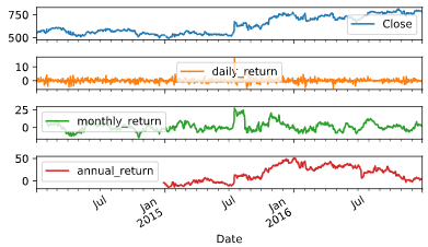
# Create daily_return
google['daily_return'] = google.Close.pct_change().mul(100)
# Create monthly_return
google['monthly_return'] = google.Close.pct_change(30).mul(100)
# Create annual_return
google['annual_return'] = google.Close.pct_change(360).mul(100)
# Plot the result
google['daily_return']
google.plot(subplots=True)
plt.show()

上面这几行的代码暴露一个问题是我的语法还是不太熟。。。

整熟了再往下学啊

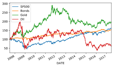
# Import data here
prices = pd.read_csv('asset_classes.csv',parse_dates=['DATE'],index_col='DATE')
# Inspect prices here
print(prices.info())
# Select first prices
first_prices = prices.iloc[0]
# Create normalized
normalized = prices.div(first_prices).mul(100)
# Plot normalized
#画图这个地方老是写错，记住直接调用
normalized.plot()
plt.show()

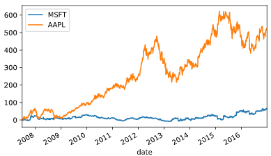
# Create tickers
tickers = ['MSFT', 'AAPL']
# Import stock data here
stocks = pd.read_csv('msft_aapl.csv', parse_dates=['date'], index_col='date')
# Import index here
sp500 = pd.read_csv('sp500.csv', parse_dates=['date'], index_col='date')
# Concatenate stocks and index here
data = pd.concat([stocks, sp500], axis=1).dropna()
# Normalize data
normalized = data.div(data.iloc[0]).mul(100)
# Subtract the normalized index from the normalized stock prices, and plot the result
normalized[tickers].sub(normalized['SP500'], axis=0).plot()
plt.show()

DataFrame.reindex()

这个函数就是重新定义索引

DataFrame.reindex(self, labels=None, index=None, columns=None, axis=None, method=None, copy=True, level=None, fill_value=nan, limit=None, tolerance=None)[source]

通过data_range指定时间序列的起止时间

# Set start and end dates
start = '2016-1-1'
end = '2016-2-29'
# Create monthly_dates here
#这个就是创建一个指定的起止时间，然后有相同的时间间隔
monthly_dates = pd.date_range(start=start, end=end, freq='M')
# Create monthly here，构造一个时间序列，但是要给一个时间戳
monthly = pd.Series(data=[1,2], index=monthly_dates)
print(monthly)
# Create weekly_dates here
weekly_dates = pd.date_range(start=start, end=end, freq='W')
# Print monthly, reindexed using weekly_dates
print(monthly.reindex(weekly_dates))
print(monthly.reindex(weekly_dates, method='bfill'))
print(monthly.reindex(weekly_dates, method='ffill'))
#ffill ： foreaward fill 向前填充，
#如果新增加索引的值不存在，那么按照前一个非nan的值填充进去
同理，bfill是后向补充
<script.py> output:
    2016-01-31    1
    2016-02-29    2
    Freq: M, dtype: int64
    2016-01-03    NaN
    2016-01-10    NaN
    2016-01-17    NaN
    2016-01-24    NaN
    2016-01-31    1.0
    2016-02-07    NaN
    2016-02-14    NaN
    2016-02-21    NaN
    2016-02-28    NaN
    Freq: W-SUN, dtype: float64
    2016-01-03    1
    2016-01-10    1
    2016-01-17    1
    2016-01-24    1
    2016-01-31    1
    2016-02-07    2
    2016-02-14    2
    2016-02-21    2
    2016-02-28    2
    Freq: W-SUN, dtype: int64
    2016-01-03    NaN
    2016-01-10    NaN
    2016-01-17    NaN
    2016-01-24    NaN
    2016-01-31    1.0
    2016-02-07    1.0
    2016-02-14    1.0
    2016-02-21    1.0
    2016-02-28    1.0
    Freq: W-SUN, dtype: float64

通过as.fred()指定时间序列的间隔

这个比较适合读入是时间序列的数据，然后直接做处理

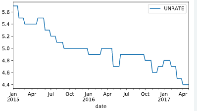
# Import data here
data = pd.read_csv('unemployment.csv', parse_dates=['date'], index_col='date')
# Show first five rows of weekly series
print(data.asfreq('W').head())
# Show first five rows of weekly series with bfill option
print(data.asfreq('W', method='bfill').head())
# Create weekly series with ffill option and show first five rows
weekly_ffill = data.asfreq('W', method='ffill')
print(weekly_ffill.head())
# Plot weekly_fill starting 2015 here
weekly_ffill.loc['2015':].plot()
plt.show()

interpolate()

这个函数是根据需求进行插值，目前的理解就是因为存在很多的缺失值进行插补，达到剔除缺失值的目的，一般情况下会暴力删除缺失值，剔除行或者列

官方文档有个demo

>>> s = pd.Series([np.nan, "single_one", np.nan,
...                "fill_two_more", np.nan, np.nan, np.nan,
...                4.71, np.nan])
>>> s
0              NaN
1       single_one
2              NaN
3    fill_two_more
4              NaN
5              NaN
6              NaN
7             4.71
8              NaN
dtype: object
>>> s.interpolate(method='pad', limit=2)
0              NaN
1       single_one
2       single_one
3    fill_two_more
4    fill_two_more
5    fill_two_more
6              NaN
7             4.71
8             4.71
dtype: object

resample()

这个函数可以给已经存在的时间序列重新划分frequency

DataFrame.resample(self, rule, how=None, axis=0, fill_method=None, closed=None, label=None, convention='start', kind=None, loffset=None, limit=None, base=0, on=None, level=None)

# Import and inspect data here
ozone = pd.read_csv('ozone.csv',parse_dates=['date'],index_col='date')
print(ozone.info())
# Calculate and plot the weekly average ozone trend
#日期的fre是week，并且求出每周的平均值
ozone.resample('W').mean().plot()
plt.show()

补充一个绘图的参数

plot(subplots=True)

这个参数代表的是有子图，且子图共用y轴

first（）

这个函数是打印指定的前几行，但是不包括end

>>> i = pd.date_range('2018-04-09', periods=4, freq='2D')
>>> ts = pd.DataFrame({'A': [1,2,3,4]}, index=i)
>>> ts
            A
2018-04-09  1
2018-04-11  2
2018-04-13  3
2018-04-15  4
Get the rows for the first 3 days:
>>> ts.first('3D')
            A
2018-04-09  1
2018-04-11  2

pct_change()

DataFrame.pct_change(periods=1, fill_method=‘pad’, limit=None, freq=None, **kwargs)

表示当前元素与先前元素的相差百分比，当然指定periods=n,表示当前元素与先前n 个元素的相差百分比

嗯，这个函数适合批量求百分比

官方文档给的例子或许更好理解

>>> df = pd.DataFrame({
...     'FR': [4.0405, 4.0963, 4.3149],
...     'GR': [1.7246, 1.7482, 1.8519],
...     'IT': [804.74, 810.01, 860.13]},
...     index=['1980-01-01', '1980-02-01', '1980-03-01'])
>>> df
                FR      GR      IT
1980-01-01  4.0405  1.7246  804.74
1980-02-01  4.0963  1.7482  810.01
1980-03-01  4.3149  1.8519  860.13
>>> df.pct_change()
                  FR        GR        IT
1980-01-01       NaN       NaN       NaN
1980-02-01  0.013810  0.013684  0.006549
1980-03-01  0.053365  0.059318  0.061876

pd.contact()

这个函数应该是类似于R 里面的rbind按行拼接，即纵向合并

>>> pd.concat([s1, s2], ignore_index=True)
0    a
1    b
2    c
3    d
dtype: object

agg()

与groupby对应的聚合函数，有点类似于summarize

将一些基础运算整合到一起

rolling window functions.

滚动窗口函数

不知道之前的garch模型滑动窗口是不是用到了这个，这个我再查一下，确实不太明白

查到了 参考：

“时点的数据波动较大，某一点的数据不能很好的表现它本身的特性，于是我们就想，能否用一个区间的的数据去表现呢，这样数据的准确性是不是更好一些呢？因此，引出滑动窗口(移动窗口)的概念，简单点说，为了提升数据的可靠性，将某个点的取值扩大到包含这个点的一段区间，用区间来进行判断，这个区间就是窗口。如下面的示意图所示，其中时间序列数据代表的是15日每日的温度，现在我们以3天为一个窗口，将这个窗口从左至右依次滑动，统计出3天的平均值作为这个点的值，比如3号的温度就是1号、2号、3号的平均温度”

DataFrame.rolling(window, min_periods=None, center=False, win_type=None, on=None, axis=0, closed=None)

• window
  
  时间窗的大小，一般有两种形式，int：表示计算统计量的观测值的数量，即向前几个数量，要是offset则表示时间窗的大小。
  
  min_periods:每个窗口最少包含的观测值的数量，小于这个窗口就是na

rolling()

join()

合并数据表的一个函数

两个DataFrame中的不同的列索引合并成为一个DataFrame

# Import and inspect ozone data here
data = pd.read_csv('ozone.csv', parse_dates=['date'], index_col='date').dropna()
# Calculate the rolling mean and std here
rolling_stats = data.Ozone.rolling(360).agg(['mean', 'std'])
# Join rolling_stats with ozone data
#默认左拼接，有点像R里面的left_join()
stats = data.join(rolling_stats)
# Plot stats
stats.plot(subplots=True);
plt.show()

quantile()

分位数函数

四分位数

概念：把给定的乱序数值由小到大排列并分成四等份，处于三个分割点位置的数值就是四分位数。

第1四分位数 (Q1)，又称“较小四分位数”，等于该样本中所有数值由小到大排列后第25%的数字。

第2四分位数 (Q2)，又称“中位数”，等于该样本中所有数值由小到大排列后第50%的数字。

第3四分位数 (Q3)，又称“较大四分位数”，等于该样本中所有数值由小到大排列后第75%的数字。

四分位距（InterQuartile Range, IQR）= 第3四分位数与第1四分位数的差距

同时拓展到多分位数的概念

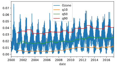
# Resample, interpolate and inspect ozone data here
data = data.resample('D').interpolate()
data.info()
# Create the rolling window
rolling = data.rolling(360)['Ozone']
# Insert the rolling quantiles to the monthly returns
data['q10'] = rolling.quantile(.1)
data['q50'] = rolling.quantile(.5)
data['q90'] = rolling.quantile(.9)
# Plot the data
data.plot()
plt.show()

append()

向dataframe对象中添加新的行，如果添加的列名不在dataframe对象中，将会被当作新的列进行添加

这个函数挺好使的 参考下官方文档 demo很好理解

可以进行行列合并

pandas 中统计累计次数

.cumsum()

累加

.cumprod()

累乘

# Import numpy
import numpy as np
# Define a multi_period_return function
def multi_period_return(period_returns):
    return np.prod(period_returns + 1) - 1
# Calculate daily returns
daily_returns = data.pct_change()
# Calculate rolling_annual_returns
rolling_annual_returns = daily_returns.rolling('360D').apply(multi_period_return)
# Plot rolling_annual_returns
rolling_annual_returns.mul(100).plot();
plt.show()

np.prod这个是numpy里面求阶乘的

# Create multi_period_return function here
def multi_period_return(r):
    return (np.prod(r + 1) - 1) * 100

定义一个函数然后直接调用就行,计算数组乘积

一个案例学习

seed()

设定种子简书

设定生成随机数的种子，种子是为了让结果具有重复性，重现结果。如果不设定种子，生成的随机数无法重现

计算机并不能产生真正的随机数，如果你不设种子，计算机会用系统时钟来作为种子，如果你要模拟什么的话，每次的随机数都是不一样的，这样就不方便你研究，如果你事先设置了种子，这样每次的随机数都是一样的，便于重现你的研究，也便于其他人检验你的分析结果

random walk

# Set seed here
seed(42)
# Create random_walk
random_walk = normal(loc=.001, scale=0.01, size=2500)
# Convert random_walk to pd.series
random_walk = pd.Series(random_walk)
# Create random_prices
random_prices = random_walk.add(1).cumprod()
# Plot random_prices here
random_prices.mul(1000).plot()
plt.show();

choice()

随机抽样函数

生成随机数

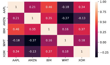
Relationships between time series: correlation

heatmap()

相关系数矩阵热力图

之前论文中读到的热图，这回终于知道该怎么画了

# Inspect data here
print(data.info())
# Calculate year-end prices here
annual_prices = data.resample('A').last()
# Calculate annual returns here
annual_returns = annual_prices.pct_change()
# Calculate and print the correlation matrix here
correlations = annual_returns.corr()
print(correlations)
# Visualize the correlations as heatmap here
sns.heatmap(correlations, annot=True)
plt.show();

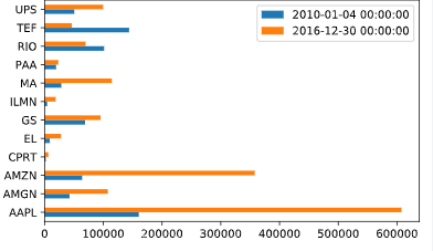
Select index components & import data

groupby()

简书

和R里面的group_by函数是一样的，好好用哦，之前写了一个for循环还是给写错了，真的是。。卧槽。。md

# Select largest company for each sector
components = listings.groupby(['Sector'])['Market Capitalization'].nlargest(1)
# Print components, sorted by market cap
print(components.sort_values(ascending=False))
# Select stock symbols and print the result
tickers = components.index.get_level_values('Stock Symbol')
print(tickers)
# Print company name, market cap, and last price for each component
info_cols = ['Company Name', 'Market Capitalization', 'Last Sale']
print(listings.loc[tickers, info_cols].sort_values('Market Capitalization', ascending=False))
<script.py> output:
    Sector                 Stock Symbol
    Technology             AAPL           740,024.47
    Consumer Services      AMZN           422,138.53
    Miscellaneous          MA             123,330.09
    Health Care            AMGN           118,927.21
    Transportation         UPS             90,180.89
    Finance                GS              88,840.59
    Basic Industries       RIO             70,431.48
    Public Utilities       TEF             54,609.81
    Consumer Non-Durables  EL              31,122.51
    Capital Goods          ILMN            25,409.38
    Energy                 PAA             22,223.00
    Consumer Durables      CPRT            13,620.92
    Name: Market Capitalization, dtype: float64
    Index(['RIO', 'ILMN', 'CPRT', 'EL', 'AMZN', 'PAA', 'GS', 'AMGN', 'MA', 'TEF', 'AAPL', 'UPS'], dtype='object', name='Stock Symbol')
                                        Company Name  Market Capitalization  Last Sale
    Stock Symbol
    AAPL                                  Apple Inc.             740,024.47     141.05
    AMZN                            Amazon.com, Inc.             422,138.53     884.67
    MA                       Mastercard Incorporated             123,330.09     111.22
    AMGN                                  Amgen Inc.             118,927.21     161.61
    UPS                  United Parcel Service, Inc.              90,180.89     103.74
    GS               Goldman Sachs Group, Inc. (The)              88,840.59     223.32
    RIO                                Rio Tinto Plc              70,431.48      38.94
    TEF                                Telefonica SA              54,609.81      10.84
    EL            Estee Lauder Companies, Inc. (The)              31,122.51      84.94
    ILMN                              Illumina, Inc.              25,409.38     173.68
    PAA           Plains All American Pipeline, L.P.              22,223.00      30.72
    CPRT                                Copart, Inc.              13,620.92      29.65

最后一行or一列的表示方法

可以用“-1”表示

sort_values

这个函数就是排序函数，类似于r里面的arrange函数

plotz中的参数kind

这个参数是用来设置绘图类型的

# Select the number of shares
no_shares = components['Number of Shares']
print(no_shares.sort_values())
# Create the series of market cap per ticker
market_cap = stock_prices.mul(no_shares)
# Select first and last market cap here
first_value = market_cap.iloc[0]
last_value = market_cap.iloc[-1]
# Concatenate and plot first and last market cap here
pd.concat([first_value, last_value], axis=1).plot(kind='barh')
plt.show()

to_excel()

将数据输出到excel中

# Export data and data as returns to excel
with pd.ExcelWriter('data.xls') as writer:
    data.to_excel(writer, sheet_name='data')
    returns.to_excel(writer, sheet_name='returns')

还行吧，记住语法，多尝试几遍就好了