【cs231n作业笔记】一：KNN分类器

安装anaconda，下载assignment作业代码

作业代码数据集等2018版基于python3.6 下载提取码4put

本课程内容参考：

cs231n官方笔记地址

贺完结！CS231n官方笔记授权翻译总集篇发布

CS231n课程笔记翻译：图像分类笔记（上）

numpy参考：CS231n课程笔记翻译：Python Numpy教程

以下文字部分转载自：

CS231n——图像分类（KNN实现）

课程作业基于python3.6.5对应的anaconda 修改了输入输出

图像分类

  目标：已有固定的分类标签集合，然后对于输入的图像，从分类标签集合中找出一个分类标签，最后把分类标签分配给该输入图像。

  图像分类流程

• 输入：输入是包含N个图像的集合，每个图像的标签是K种分类标签中的一种。这个集合称为训练集。
• 学习：这一步的任务是使用训练集来学习每个类到底长什么样。一般该步骤叫做训练分类器或者学习一个模型。
• 评价：让分类器来预测它未曾见过的图像的分类标签，把分类器预测的标签和图像真正的分类标签对比，并以此来评价分类器的质量。

  Nearest Neighbor分类器

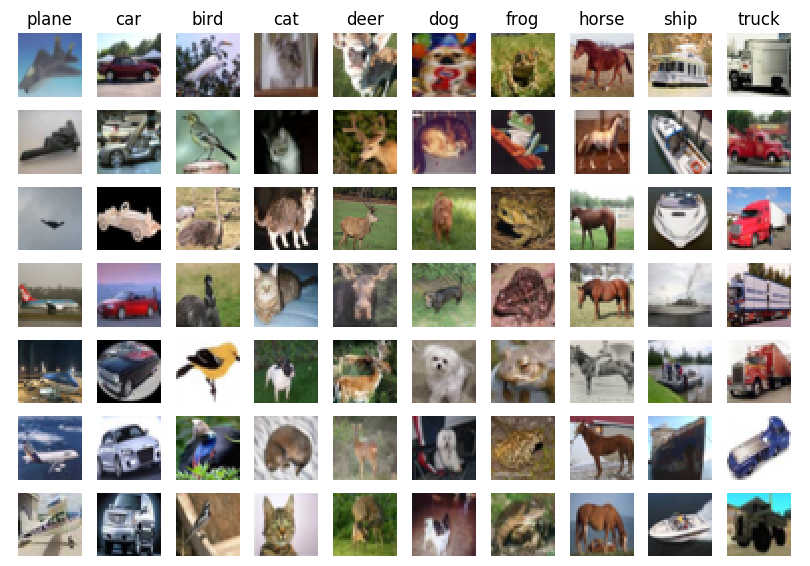
  数据集：CIFAR-10。这是一个非常流行的图像分类数据集，包含了60000张32X32的小图像。每张图像都有10种分类标签中的一种。这60000张图像被分为包含50000张图像的训练集和包含10000张图像的测试集。

  Nearest Neighbor图像分类思想：拿测试图片和训练集中每一张图片去比较，然后将它认为最相似的那个训练集图片的标签赋给这张测试图片。
  如何比较来那个张图片？
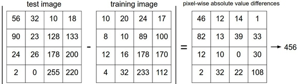
  在本例中，就是比较32x32x3的像素块。最简单的方法就是逐个像素比较，最后将差异值全部加起来。换句话说，就是将两张图片先转化为两个向量I_1和I_2，然后计算他们的L1距离：

这里的求和是针对所有的像素。下面是整个比较流程的图例：

  计算向量间的距离有很多种方法，另一个常用的方法是L2距离，从几何学的角度，可以理解为它在计算两个向量间的欧式距离。L2距离的公式如下：

  L1和L2比较：比较这两个度量方式是挺有意思的。在面对两个向量之间的差异时，L2比L1更加不能容忍这些差异。也就是说，相对于1个巨大的差异，L2距离更倾向于接受多个中等程度的差异。L1和L2都是在p-norm常用的特殊形式。

  k-Nearest Neighbor分类器(KNN)

  KNN图像分类思想：与其只找最相近的那1个图片的标签，我们找最相似的k个图片的标签，然后让他们针对测试图片进行投票，最后把票数最高的标签作为对测试图片的预测。
  如何选择k值？
  交叉验证：假如有1000张图片，我们将训练集平均分成5份，其中4份用来训练，1份用来验证。然后我们循环着取其中4份来训练，其中1份来验证，最后取所有5次验证结果的平均值作为算法验证结果。

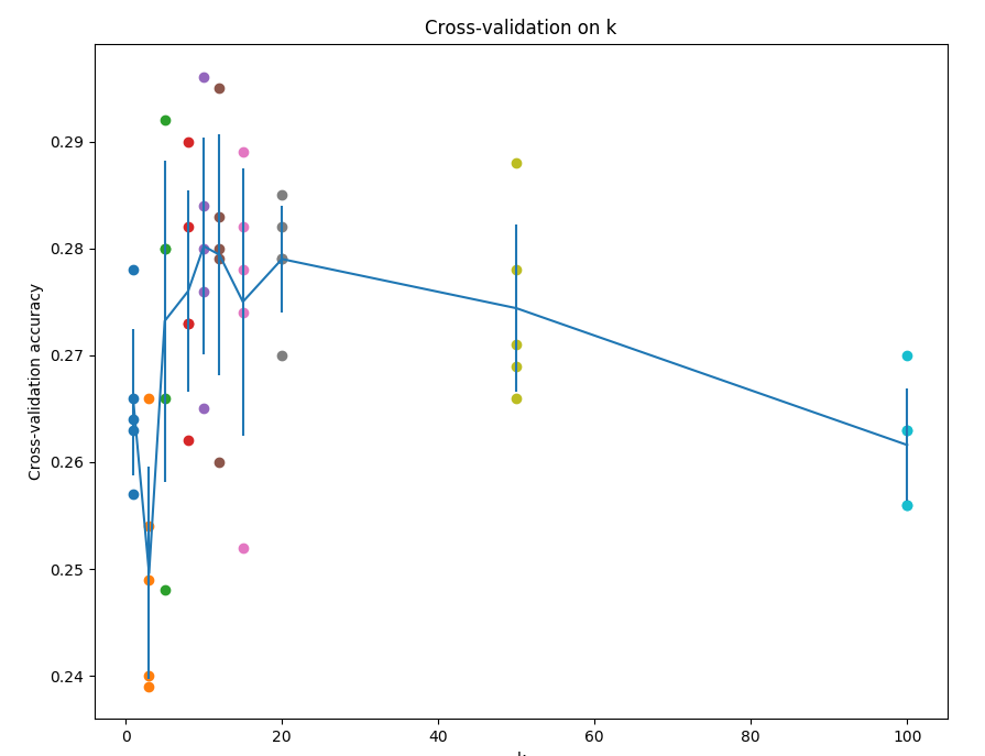
  这就是5份交叉验证对k值调优的例子。针对每个k值，得到5个准确率结果，取其平均值，然后对不同k值的平均表现画线连接。本例中，当k=10的时算法表现最好（对应图中的准确率峰值）。如果我们将训练集分成更多份数，直线一般会更加平滑（噪音更少）。

  k-Nearest Neighbor分类器的优劣

  优点：

• 思路清晰，易于理解，实现简单；
• 算法的训练不需要花时间，因为其训练过程只是将训练集数据存储起来。

  缺点：测试要花费大量时间计算，因为每个测试图像需要和所有存储的训练图像进行比较。

  实际应用k-NN

  如果你希望将k-NN分类器用到实处（最好别用到图像上，若是仅仅作为练手还可以接受），那么可以按照以下流程：

1. 预处理你的数据：对你数据中的特征进行归一化（normalize），让其具有零平均值（zero mean）和单位方差（unit variance）。在后面的小节我们会讨论这些细节。本小节不讨论，是因为图像中的像素都是同质的，不会表现出较大的差异分布，也就不需要标准化处理了。
2. 如果数据是高维数据，考虑使用降维方法，比如PCA(wiki ref, CS229ref, blog ref)或随机投影。
3. 将数据随机分入训练集和验证集。按照一般规律，70%-90% 数据作为训练集。这个比例根据算法中有多少超参数，以及这些超参数对于算法的预期影响来决定。如果需要预测的超参数很多，那么就应该使用更大的验证集来有效地估计它们。如果担心验证集数量不够，那么就尝试交叉验证方法。如果计算资源足够，使用交叉验证总是更加安全的（份数越多，效果越好，也更耗费计算资源）。
4. 在验证集上调优，尝试足够多的k值，尝试L1和L2两种范数计算方式。
5. 如果分类器跑得太慢，尝试使用Approximate Nearest Neighbor库（比如FLANN）来加速这个过程，其代价是降低一些准确率。
6. 对最优的超参数做记录。记录最优参数后，是否应该让使用最优参数的算法在完整的训练集上运行并再次训练呢？因为如果把验证集重新放回到训练集中（自然训练集的数据量就又变大了），有可能最优参数又会有所变化。在实践中，不要这样做。千万不要在最终的分类器中使用验证集数据，这样做会破坏对于最优参数的估计。直接使用测试集来测试用最优参数设置好的最优模型，得到测试集数据的分类准确率，并以此作为你的kNN分类器在该数据上的性能表现。

  课程作业

课程作业：assignment 1

主函数knn.py 放在根目录assignment下

#coding:utf-8
'''
#knn.py
Created on 2019年4月11日

@author: Joel
'''
import random
import numpy as np
from assignment1.data_utils import load_CIFAR10
from  assignment1.classifiers.k_nearest_neighbor import KNearestNeighbor
import matplotlib.pyplot as plt

# This is a bit of magic to make matplotlib figures appear inline in the notebook
# rather than in a new window.
plt.rcParams['figure.figsize'] = (10.0, 8.0) # set default size of plots
plt.rcParams['image.interpolation'] = 'nearest'
plt.rcParams['image.cmap'] = 'gray'

X_train, y_train, X_test, y_test = load_CIFAR10('../datasets')

# As a sanity check, we print out the size of the training and test data.
print('Training data shape: ', X_train.shape)
print('Training labels shape: ', y_train.shape)
print('Test data shape: ', X_test.shape)
print('Test labels shape: ', y_test.shape)

# 从数据集中展示一部分数据
# 每个类别展示若干张对应图片
classes = ['plane', 'car', 'bird', 'cat', 'deer', 'dog', 'frog', 'horse', 'ship', 'truck']
num_classes = len(classes)
samples_per_class = 7
for y, cls in enumerate(classes):
    idxs = np.flatnonzero(y_train == y)
    idxs = np.random.choice(idxs, samples_per_class, replace=False)
    for i, idx in enumerate(idxs):
        plt_idx = i * num_classes + y + 1
        plt.subplot(samples_per_class, num_classes, plt_idx)
        plt.imshow(X_train[idx].astype('uint8'))
        plt.axis('off')
        if i == 0:
            plt.title(cls)
plt.show()

# 截取部分样本数据，以提高本作业的执行效率
num_training = 5000
mask = range(num_training)
X_train = X_train[mask]
y_train = y_train[mask]

num_test = 500
mask = range(num_test)
X_test = X_test[mask]
y_test = y_test[mask]

# reshape训练和测试数据，转换为行的形式
X_train = np.reshape(X_train, (X_train.shape[0], -1))
X_test = np.reshape(X_test, (X_test.shape[0], -1))

print(X_train.shape)
print(X_test.shape)

classifier = KNearestNeighbor()
classifier.train(X_train, y_train)

dists = classifier.compute_distances_two_loops(X_test)
print(dists.shape)

plt.imshow(dists, interpolation='none')
plt.show()

# Now implement the function predict_labels and run the code below:
# k=1时
y_test_pred = classifier.predict_labels(dists, k=1)

# Compute and print the fraction of correctly predicted examples
num_correct = np.sum(y_test_pred == y_test)
accuracy = float(num_correct) / num_test
print('Got %d / %d correct => accuracy: %f' % (num_correct, num_test, accuracy))

# k=5时
y_test_pred = classifier.predict_labels(dists, k=5)
num_correct = np.sum(y_test_pred == y_test)
accuracy = float(num_correct) / num_test
print('Got %d / %d correct => accuracy: %f' % (num_correct, num_test, accuracy))

####测试三种距离计算法的效率

dists_one = classifier.compute_distances_one_loop(X_test)

difference = np.linalg.norm(dists - dists_one, ord='fro')
print('Difference was: %f' % (difference, ))
if difference < 0.001:
  print('Good! The distance matrices are the same')
else:
  print('Uh-oh! The distance matrices are different')

dists_two = classifier.compute_distances_no_loops(X_test)
difference = np.linalg.norm(dists - dists_two, ord='fro')
print('Difference was: %f' % (difference, ))
if difference < 0.001:
  print('Good! The distance matrices are the same')
else:
  print('Uh-oh! The distance matrices are different')

def time_function(f, *args):
  """
  Call a function f with args and return the time (in seconds) that it took to execute.
  """
  import time
  tic = time.time()
  f(*args)
  toc = time.time()
  return toc - tic

two_loop_time = time_function(classifier.compute_distances_two_loops, X_test)
print('Two loop version took %f seconds' % two_loop_time)

one_loop_time = time_function(classifier.compute_distances_one_loop, X_test)
print('One loop version took %f seconds' % one_loop_time)

no_loop_time = time_function(classifier.compute_distances_no_loops, X_test)
print('No loop version took %f seconds' % no_loop_time)

# 交叉验证
num_folds = 5
k_choices = [1, 3, 5, 8, 10, 12, 15, 20, 50, 100]

X_train_folds = []
y_train_folds = []
################################################################################
# TODO:                                                                        #
# Split up the training data into folds. After splitting, X_train_folds and    #
# y_train_folds should each be lists of length num_folds, where                #
# y_train_folds[i] is the label vector for the points in X_train_folds[i].     #
# Hint: Look up the numpy array_split function.                                #
################################################################################
#数据划分
X_train_folds = np.array_split(X_train, num_folds);
y_train_folds = np.array_split(y_train, num_folds)
################################################################################
#                                 END OF YOUR CODE                             #
################################################################################

# A dictionary holding the accuracies for different values of k that we find
# when running cross-validation. After running cross-validation,
# k_to_accuracies[k] should be a list of length num_folds giving the different
# accuracy values that we found when using that value of k.

k_to_accuracies = {}

################################################################################
# TODO:                                                                        #
# Perform k-fold cross validation to find the best value of k. For each        #
# possible value of k, run the k-nearest-neighbor algorithm num_folds times,   #
# where in each case you use all but one of the folds as training data and the #
# last fold as a validation set. Store the accuracies for all fold and all     #
# values of k in the k_to_accuracies dictionary.                               #
################################################################################
for k in k_choices:
    k_to_accuracies[k] = []

for k in k_choices:#find the best k-value
    for i in range(num_folds):
        X_train_cv = np.vstack(X_train_folds[:i]+X_train_folds[i+1:])
        X_test_cv = X_train_folds[i]

        y_train_cv = np.hstack(y_train_folds[:i]+y_train_folds[i+1:])  #size:4000
        y_test_cv = y_train_folds[i]

        classifier.train(X_train_cv, y_train_cv)
        dists_cv = classifier.compute_distances_no_loops(X_test_cv)

        y_test_pred = classifier.predict_labels(dists_cv, k)
        num_correct = np.sum(y_test_pred == y_test_cv)
        accuracy = float(num_correct) / y_test_cv.shape[0]

        k_to_accuracies[k].append(accuracy)
################################################################################
#                                 END OF YOUR CODE                             #
################################################################################

# Print out the computed accuracies
for k in sorted(k_to_accuracies):
    for accuracy in k_to_accuracies[k]:
        print('k = %d, accuracy = %f' % (k, accuracy))

# plot the raw observations
for k in k_choices:
  accuracies = k_to_accuracies[k]
  plt.scatter([k] * len(accuracies), accuracies)

# plot the trend line with error bars that correspond to standard deviation
accuracies_mean = np.array([np.mean(v) for k,v in sorted(k_to_accuracies.items())])
accuracies_std = np.array([np.std(v) for k,v in sorted(k_to_accuracies.items())])
plt.errorbar(k_choices, accuracies_mean, yerr=accuracies_std)
plt.title('Cross-validation on k')
plt.xlabel('k')
plt.ylabel('Cross-validation accuracy')
plt.show()

# Based on the cross-validation results above, choose the best value for k,
# retrain the classifier using all the training data, and test it on the test
# data. You should be able to get above 28% accuracy on the test data.
best_k = 10

classifier = KNearestNeighbor()
classifier.train(X_train, y_train)
y_test_pred = classifier.predict(X_test, k=best_k)

# Compute and display the accuracy
num_correct = np.sum(y_test_pred == y_test)
accuracy = float(num_correct) / num_test
print ('Got %d / %d correct => accuracy: %f' % (num_correct, num_test, accuracy))

assignment.cs231n.classifiers目录

k_nearest_neighbor.py文件内容：

主要是完成了KNN分类器预测部分，分别用了双层循环，已经运用numpy广播的无循环和单循环计算，广播方法的无循环最快；

预测label的选择，选择k个离样本最近的下标，选择出现次数最多的下标作为测试样本的分类；

通过将训练样本分成5部分对k的不同取值进行交叉验证，最终选择分类效果最好的k，结果为k=12；

np.bincount:统计每个元素出现的次数,np.argmax()将次数出现最多的下标返回；

numpy.argsort()返回数组值从小到大的索引； [:k]为返回最小的k个距离；

#coding:utf-8

#k_nearest_neighbor.py

import numpy as np

class KNearestNeighbor(object):
  """ a kNN classifier with L2 distance """

  def __init__(self):
    pass

  def train(self, X, y):
    """
    Train the classifier. For k-nearest neighbors this is just
    memorizing the training data.

    Inputs:
    - X: A numpy array of shape (num_train, D) containing the training data
      consisting of num_train samples each of dimension D.
    - y: A numpy array of shape (N,) containing the training labels, where
         y[i] is the label for X[i].
    """
    self.X_train = X
    self.y_train = y

  def predict(self, X, k=1, num_loops=0):
    """
    Predict labels for test data using this classifier.

    Inputs:
    - X: A numpy array of shape (num_test, D) containing test data consisting
         of num_test samples each of dimension D.
    - k: The number of nearest neighbors that vote for the predicted labels.
    - num_loops: Determines which implementation to use to compute distances
      between training points and testing points.

    Returns:
    - y: A numpy array of shape (num_test,) containing predicted labels for the
      test data, where y[i] is the predicted label for the test point X[i].
    """
    if num_loops == 0:
      dists = self.compute_distances_no_loops(X)
    elif num_loops == 1:
      dists = self.compute_distances_one_loop(X)
    elif num_loops == 2:
      dists = self.compute_distances_two_loops(X)
    else:
      raise ValueError('Invalid value %d for num_loops' % num_loops)

    return self.predict_labels(dists, k=k)

  def compute_distances_two_loops(self, X):
    """
    Compute the distance between each test point in X and each training point
    in self.X_train using a nested loop over both the training data and the
    test data.

    Inputs:
    - X: A numpy array of shape (num_test, D) containing test data.

    Returns:
    - dists: A numpy array of shape (num_test, num_train) where dists[i, j]
      is the Euclidean distance between the ith test point and the jth training
      point.
    """
    num_test = X.shape[0]
    num_train = self.X_train.shape[0]
    dists = np.zeros((num_test, num_train))
    for i in range(num_test):
      for j in range(num_train):
        #####################################################################
        # TODO:                                                             #
        # Compute the l2 distance between the ith test point and the jth    #
        # training point, and store the result in dists[i, j]. You should   #
        # not use a loop over dimension.                                    #
        #####################################################################
        dists[i][j]=np.sqrt(np.sum(np.square(self.X_train[j,:]-X[i,:])))
        #####################################################################
        #                       END OF YOUR CODE                            #
        #####################################################################
    return dists

  def compute_distances_one_loop(self, X):
    """
    Compute the distance between each test point in X and each training point
    in self.X_train using a single loop over the test data.

    Input / Output: Same as compute_distances_two_loops
    """
    num_test = X.shape[0]
    num_train = self.X_train.shape[0]
    dists = np.zeros((num_test, num_train))
    for i in range(num_test):
      #######################################################################
      # TODO:                                                               #
      # Compute the l2 distance between the ith test point and all training #
      # points, and store the result in dists[i, :].                        #
      #######################################################################
      dists[i,:]=np.sqrt(np.sum(np.square(self.X_train-X[i,:]),axis=1))
      #######################################################################
      #                         END OF YOUR CODE                            #
      #######################################################################
    return dists

  def compute_distances_no_loops(self, X):
    """
    Compute the distance between each test point in X and each training point
    in self.X_train using no explicit loops.

    Input / Output: Same as compute_distances_two_loops
    """
    num_test = X.shape[0]
    num_train = self.X_train.shape[0]
    dists = np.zeros((num_test, num_train))
    #########################################################################
    # TODO:                                                                 #
    # Compute the l2 distance between all test points and all training      #
    # points without using any explicit loops, and store the result in      #
    # dists.                                                                #
    #                                                                       #
    # You should implement this function using only basic array operations; #
    # in particular you should not use functions from scipy.                #
    #                                                                       #
    # HINT: Try to formulate the l2 distance using matrix multiplication    #
    #       and two broadcast sums.
    # 矩阵广播求和的方法                                        #
    #########################################################################
    ab=np.dot(X,self.X_train.T)
    a_2=np.square(X).sum(axis=1)
    b_2=np.square(self.X_train).sum(axis=1)
    print(ab.shape)
    print(a_2.shape)
    print(b_2.shape)
    dists_2=-2*ab+b_2+np.matrix(a_2).T
    dists=np.array(np.sqrt(dists_2))
    #########################################################################
    #                         END OF YOUR CODE                              #
    #########################################################################
    return dists

  def predict_labels(self, dists, k=1):
    """
    Given a matrix of distances between test points and training points,
    predict a label for each test point.

    Inputs:
    - dists: A numpy array of shape (num_test, num_train) where dists[i, j]
      gives the distance betwen the ith test point and the jth training point.

    Returns:
    - y: A numpy array of shape (num_test,) containing predicted labels for the
      test data, where y[i] is the predicted label for the test point X[i].
    """
    num_test = dists.shape[0]
    y_pred = np.zeros(num_test)
    for i in range(num_test):
      # A list of length k storing the labels of the k nearest neighbors to
      # the ith test point.
      closest_y = []
      #########################################################################
      # TODO:                                                                 #
      # Use the distance matrix to find the k nearest neighbors of the ith    #
      # testing point, and use self.y_train to find the labels of these       #
      # neighbors. Store these labels in closest_y.                           #
      # Hint: Look up the function numpy.argsort.
      # numpy.argsort()返回数组值从小到大的索引； [:k]为返回最小的k个距离；                           #
      #########################################################################
      closest_y=self.y_train[np.argsort(dists[i,:])[:k]]
      #########################################################################
      # TODO:                                                                 #
      # Now that you have found the labels of the k nearest neighbors, you    #
      # need to find the most common label in the list closest_y of labels.   #
      # Store this label in y_pred[i]. Break ties by choosing the smaller     #
      # label.    np.bincount:统计每个元素出现的次数,np.argmax()将次数出现最多的下标返回；                                                            #
      #########################################################################
      y_pred[i]=np.argmax(np.bincount(closest_y))
      #########################################################################
      #                           END OF YOUR CODE                            #
      #########################################################################

    return y_pred