深度学习之step by step搭建神经网络

声明

本文参考Deep-Learning-Specialization-Coursera/Convolution_model_Step_by_Step_v1.ipynb at main · abdur75648/Deep-Learning-Specialization-Coursera · GitHub，力求理解。

---

资料下载

链接：https://pan.baidu.com/s/1LoMe9bS_ig0wB7ubR9m39Q
提取码：afhc，请在开始之前下载好所需资料。

---

【博主使用的python版本：3.9.12】，当然也使用tensorflow2.

---

1. 神经网络的底层搭建

  这里，我们要实现一个拥有卷积层（CONV）和池化层（POOL）的网络，它包含了前向和反向传播。

nH,nW,nc,是指分别表示给定层的图像的高度、宽度和通道数。如果你想特指某一层，那么可以这样写：nH[L],nW[L],nc[L]

1 - Packages

我们先要引入一些库：

import numpy as np
import h5py
import matplotlib.pyplot as plt
from public_tests import *

%matplotlib inline
plt.rcParams['figure.figsize'] = (5.0, 4.0) # set default size of plots
plt.rcParams['image.interpolation'] = 'nearest'
plt.rcParams['image.cmap'] = 'gray'

np.random.seed(1)

2 - Outline of the Assignment

我们将实现一个卷积神经网络的一些模块，下面我们将列举我们要实现的模块的函数功能：

1. 卷积模块，包含了以下函数：

• 使用0扩充边界
• 卷积窗口
• 前向卷积
• 反向卷积（可选）

　　  2.池化模块，包含了以下函数：

• 前向池化
• 创建掩码
• 值分配
• 反向池化（可选）
• 我们将在这里从底层搭建一个完整的模块，之后我们会用TensorFlow实现。模型结构如下：

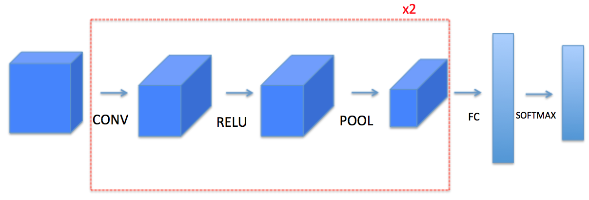
需要注意的是我们在前向传播的过程中，我们会存储一些值，以便在反向传播的过程中计算梯度值。

3 - Convolutional Neural Networks

尽管编程框架使卷积容易使用，但它们仍然是深度学习中最难理解的概念之一。卷积层将输入转换成不同维度的输出，如下所示。

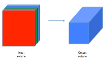
我们将一步步构建卷积层，我们将首先实现两个辅助函数：一个用于零填充，另一个用于计算卷积。

3.1 - Zero-Padding

边界填充将会在图像边界周围添加值为0的像素点，如下图所示：

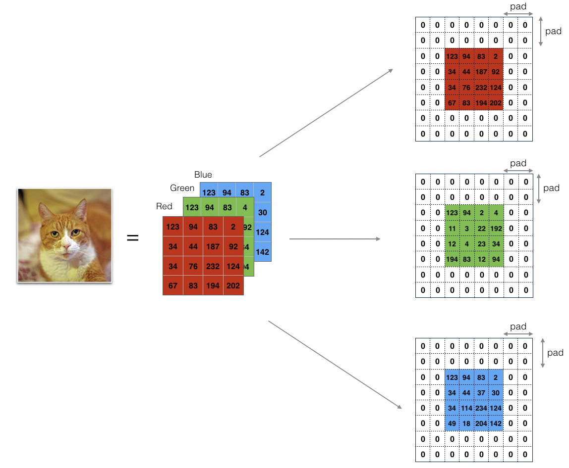
使用0填充边界有以下好处：

卷积了上一层之后的CONV层，没有缩小高度和宽度。 这对于建立更深的网络非常重要，否则在更深层时，高度/宽度会缩小。 一个重要的例子是“same”卷积，其中高度/宽度在卷积完一层之后会被完全保留。

它可以帮助我们在图像边界保留更多信息。在没有填充的情况下，卷积过程中图像边缘的极少数值会受到过滤器的影响从而导致信息丢失。

  我们将实现一个边界填充函数，它会把所有的样本图像X XX都使用0进行填充。我们可以使用np.pad来快速填充。需要注意的是如果你想使用pad = 1填充数组**a**.shape = ( 5 , 5 , 5 , 5 , 5 )的第二维，使用pad = 3填充第4维，使用pad = 0来填充剩下的部分，我们可以这么做：

a = np.pad(a, ((0,0), (1,1), (0,0), (3,3), (0,0)), mode='constant', constant_values = (0,0))

def zero_pad(X,pad):
    """
    把数据集X的图像边界全部使用0来扩充pad个宽度和高度。

    参数：
        X - 图像数据集，维度为（样本数，图像高度，图像宽度，图像通道数）
        pad - 整数，每个图像在垂直和水平维度上的填充量
    返回：
        X_paded - 扩充后的图像数据集，维度为（样本数，图像高度 + 2*pad，图像宽度 + 2*pad，图像通道数）

    """

    X_paded = np.pad(X,(
                        (0,0),       #样本数，不填充
                        (pad,pad),   #图像高度,你可以视为上面填充x个，下面填充y个(x,y)
                        (pad,pad),   #图像宽度,你可以视为左边填充x个，右边填充y个(x,y)
                        (0,0)),      #通道数，不填充
                        'constant', constant_values=0)      #连续一样的值填充

    return X_paded
                            

我们来测试一下：

np.random.seed(1)
x = np.random.randn(4, 3, 3, 2)
x_pad = zero_pad(x, 3)
print ("x.shape =\n", x.shape)
print ("x_pad.shape =\n", x_pad.shape)
print ("x[1,1] =\n", x[1, 1])
print ("x_pad[1,1] =\n", x_pad[1, 1])

assert type(x_pad) == np.ndarray, "输出必须是numpy数组"
assert x_pad.shape == (4, 9, 9, 2), f"Wrong shape: {x_pad.shape} != (4, 9, 9, 2)"
print(x_pad[0, 0:2,:, 0]) # 查看第0行到第1行的数据
assert np.allclose(x_pad[0, 0:2,:, 0], [[0, 0, 0, 0, 0, 0, 0, 0, 0], [0, 0, 0, 0, 0, 0, 0, 0, 0]], 1e-15), "Rows are not padded with zeros"
assert np.allclose(x_pad[0, :, 7:9, 1].transpose(), [[0, 0, 0, 0, 0, 0, 0, 0, 0], [0, 0, 0, 0, 0, 0, 0, 0, 0]], 1e-15), "Columns are not padded with zeros"
assert np.allclose(x_pad[:, 3:6, 3:6, :], x, 1e-15), "Internal values are different"

#绘图
fig, axarr = plt.subplots(1, 2)
axarr[0].set_title('x')
axarr[0].imshow(x[0, :, :, 0])
axarr[1].set_title('x_pad')
axarr[1].imshow(x_pad[0, :, :, 0])

3.2 - Single Step of Convolution

在这里，我们要实现第一步卷积，我们要使用一个过滤器来卷积输入的数据。先来看看下面的这个gif：

在计算机视觉应用中，左侧矩阵中的每个值都对应一个像素值，我们通过将其值与原始矩阵元素相乘，然后对它们进行求和来将3x3滤波器与图像进行卷积。我们需要实现一个函数，可以将一个3x3滤波器与单独的切片块进行卷积并输出一个实数。现在我们开始实现conv_single_step()

def conv_single_step(a_slice_prev, W, b):
    """
    在前一层的激活输出的一个片段上应用一个由参数W定义的过滤器。
    这里切片大小和过滤器大小相同

    参数：
        a_slice_prev - 输入数据的一个片段，维度为（过滤器大小，过滤器大小，上一通道数）
        W - 权重参数，包含在了一个矩阵中，维度为（过滤器大小，过滤器大小，上一通道数）
        b - 偏置参数，包含在了一个矩阵中，维度为（1,1,1）

    返回：
        Z - 在输入数据的片X上卷积滑动窗口（w，b）的结果。
    """
    s = np.multiply(a_slice_prev,W)
    # Sum over all entries of the volume s.
    Z = np.sum(s)
    # Add bias b to Z. Cast b to a float() so that Z results in a scalar value.
    b = np.squeeze(b)
    Z = Z + b

    return Z

我们来测试一下：

np.random.seed(1)
a_slice_prev = np.random.randn(4, 4, 3)
W = np.random.randn(4, 4, 3)
b = np.random.randn(1, 1, 1)

Z = conv_single_step(a_slice_prev, W, b)
print("Z =", Z)

assert (type(Z) == np.float64 or type(Z) == np.float32), "You must cast the output to float"

Z = -6.999089450680221

3.3 - Convolutional Neural Networks - Forward Pass

在前向传播的过程中，我们将使用多种过滤器对输入的数据进行卷积操作，每个过滤器会产生一个2D的矩阵，我们可以把它们堆叠起来，于是这些2D的卷积矩阵就变成了高维的矩阵。我们可以看一下下面的图：

如果我想要自定义切片，我们可以这么做：先定义要切片的位置，vert_start、vert_end、 horiz_start、 horiz_end，它们的位置我们看一下下面的图就明白了。

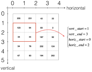
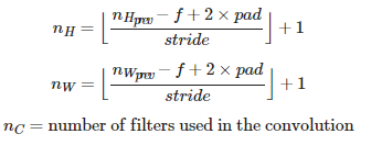
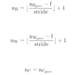
我们还是说一下输出的维度的计算公式吧~

这里我们使用for循环

def conv_forward(A_prev, W, b, hparameters):
    """
    实现卷积函数的前向传播

    参数：
        A_prev - 上一层的激活输出矩阵，维度为(m, n_H_prev, n_W_prev, n_C_prev)，（样本数量，上一层图像的高度，上一层图像的宽度，上一层过滤器数量）
        W - 权重矩阵，维度为(f, f, n_C_prev, n_C)，（过滤器大小，过滤器大小，上一层的过滤器数量，这一层的过滤器数量）
        b - 偏置矩阵，维度为(1, 1, 1, n_C)，（1,1,1,这一层的过滤器数量）
        hparameters - 包含了"stride"与 "pad"的超参数字典。

    返回：
        Z - 卷积输出，维度为(m, n_H, n_W, n_C)，（样本数，图像的高度，图像的宽度，过滤器数量）
        cache - 缓存了一些反向传播函数conv_backward()需要的一些数据
    """

    #获取来自上一层数据的基本信息
    (m , n_H_prev , n_W_prev , n_C_prev) = A_prev.shape

    #获取权重矩阵的基本信息
    ( f , f ,n_C_prev , n_C ) = W.shape

    #获取超参数hparameters的值
    stride = hparameters["stride"]
    pad = hparameters["pad"]

    #计算卷积后的图像的宽度高度，参考上面的公式，使用int()来进行板除
    n_H = int(( n_H_prev - f + 2 * pad )/ stride) + 1
    n_W = int(( n_W_prev - f + 2 * pad )/ stride) + 1

    #使用0来初始化卷积输出Z
    Z = np.zeros((m,n_H,n_W,n_C))

    #通过A_prev创建填充过了的A_prev_pad
    A_prev_pad = zero_pad(A_prev,pad)

    for i in range(m):                              #遍历样本
        a_prev_pad = A_prev_pad[i]                  #选择第i个样本的扩充后的激活矩阵
        for h in range(n_H):                        #在输出的垂直轴上循环
            for w in range(n_W):                    #在输出的水平轴上循环
                for c in range(n_C):                #循环遍历输出的通道
                    #定位当前的切片位置
                    vert_start = h * stride         #竖向，开始的位置
                    vert_end = vert_start + f       #竖向，结束的位置
                    horiz_start = w * stride        #横向，开始的位置
                    horiz_end = horiz_start + f     #横向，结束的位置
                    #切片位置定位好了我们就把它取出来,需要注意的是我们是“穿透”取出来的，
                    #自行脑补一下吸管插入一层层的橡皮泥就明白了
                    a_slice_prev = a_prev_pad[vert_start:vert_end,horiz_start:horiz_end,:]
                    #执行单步卷积
                    Z[i,h,w,c] = conv_single_step(a_slice_prev,W[: ,: ,: ,c],b[0,0,0,c])

    #数据处理完毕，验证数据格式是否正确
    assert(Z.shape == (m , n_H , n_W , n_C ))

    #存储一些缓存值，以便于反向传播使用
    cache = (A_prev,W,b,hparameters)

    return (Z , cache)

我们来测试一下;

np.random.seed(1)
A_prev = np.random.randn(2, 5, 5, 3)
hparameters = {"stride" : 1, "f": 3}

A, cache = pool_forward(A_prev, hparameters, mode = "max")
print("mode = max")
print("A.shape = " + str(A.shape))
print("A[1, 1] =\n", A[1, 1])
print()
A, cache = pool_forward(A_prev, hparameters, mode = "average")
print("mode = average")
print("A.shape = " + str(A.shape))
print("A[1, 1] =\n", A[1, 1])

Z's mean =
 0.5511276474566768
Z[0,2,1] =
 [-2.17796037  8.07171329 -0.5772704   3.36286738  4.48113645 -2.89198428
 10.99288867  3.03171932]
cache_conv[0][1][2][3] =
 [-1.1191154   1.9560789  -0.3264995  -1.34267579]

Finally, a CONV layer should also contain an activation, in which case you would add the following line of code:

# Convolve the window to get back one output neuron
Z[i, h, w, c] = ...
# Apply activation
A[i, h, w, c] = activation(Z[i, h, w, c])

You don't need to do it here, however.

4 - Pooling Layer

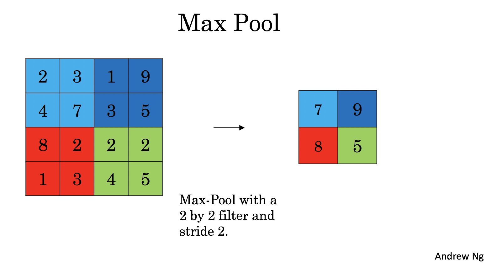
池化层会减少输入的宽度和高度，这样它会较少计算量的同时也使特征检测器对其在输入中的位置更加稳定。下面介绍两种类型的池化层：

• 最大值池化层：在输入矩阵中滑动一个大小为fxf的窗口，选取窗口里的值中的最大值，然后作为输出的一部分。
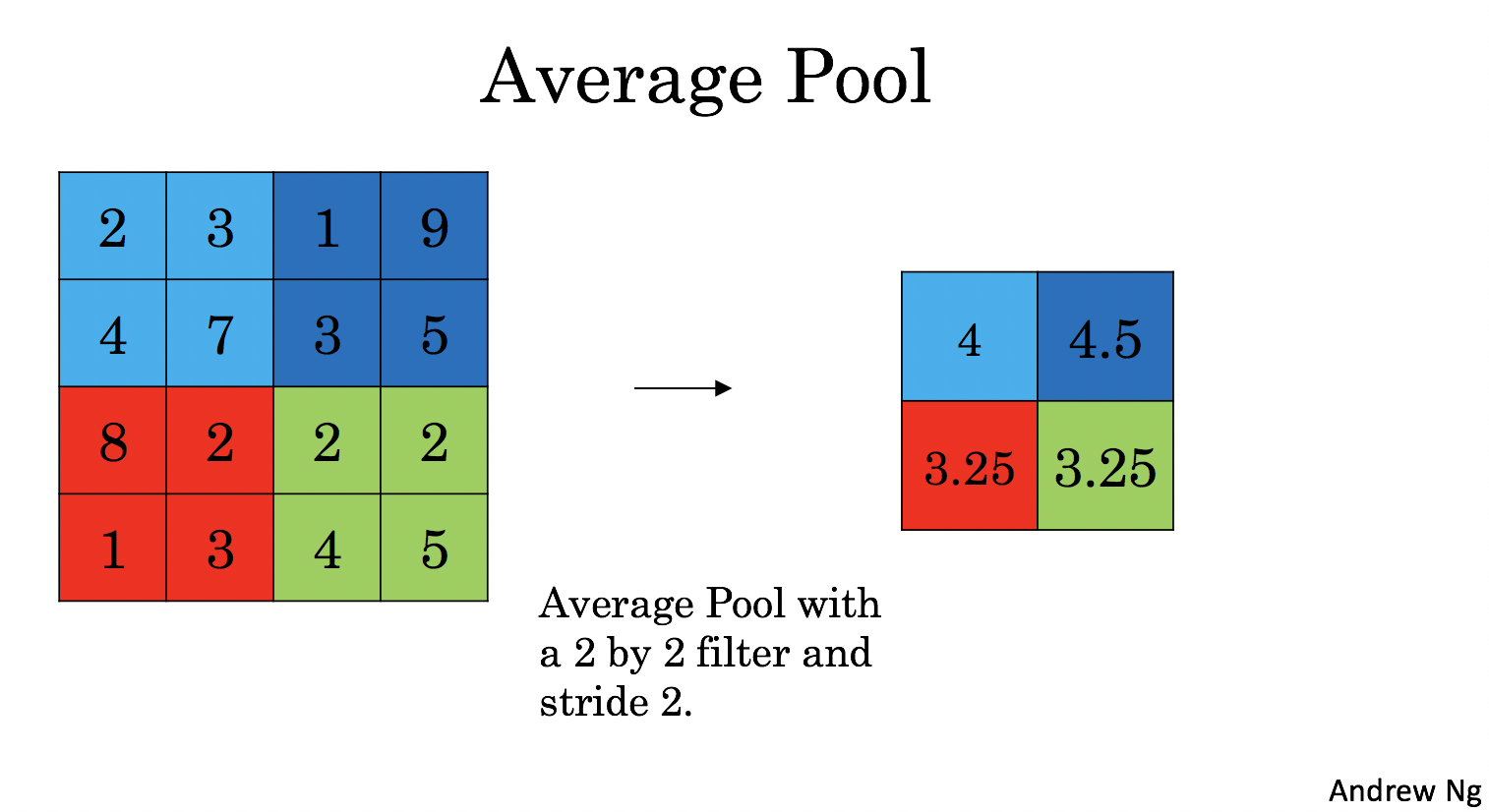
• 均值池化层：在输入矩阵中滑动一个大小为fxf的窗口，计算窗口里的值中的平均值，然后这个均值作为输出的一部分。

4.1 - Forward Pooling

def pool_forward(A_prev,hparameters,mode="max"):
    """
    实现池化层的前向传播

    参数：
        A_prev - 输入数据，维度为(m, n_H_prev, n_W_prev, n_C_prev)
        hparameters - 包含了 "f" 和 "stride"的超参数字典
        mode - 模式选择【"max" | "average"】

    返回：
        A - 池化层的输出，维度为 (m, n_H, n_W, n_C)
        cache - 存储了一些反向传播需要用到的值，包含了输入和超参数的字典。
    """

    #获取输入数据的基本信息
    (m , n_H_prev , n_W_prev , n_C_prev) = A_prev.shape

    #获取超参数的信息
    f = hparameters["f"]
    stride = hparameters["stride"]

    #计算输出维度
    n_H = int((n_H_prev - f) / stride ) + 1
    n_W = int((n_W_prev - f) / stride ) + 1
    n_C = n_C_prev

    #初始化输出矩阵
    A = np.zeros((m , n_H , n_W , n_C))

    for i in range(m):                              #遍历样本
        for h in range(n_H):                        #在输出的垂直轴上循环
            for w in range(n_W):                    #在输出的水平轴上循环
                for c in range(n_C):                #循环遍历输出的通道
                    #定位当前的切片位置
                    vert_start = h * stride         #竖向，开始的位置
                    vert_end = vert_start + f       #竖向，结束的位置
                    horiz_start = w * stride        #横向，开始的位置
                    horiz_end = horiz_start + f     #横向，结束的位置
                    #定位完毕，开始切割
                    a_slice_prev = A_prev[i,vert_start:vert_end,horiz_start:horiz_end,c]

                    #对切片进行池化操作
                    if mode == "max":
                        A[ i , h , w , c ] = np.max(a_slice_prev)
                    elif mode == "average":
                        A[ i , h , w , c ] = np.mean(a_slice_prev)

    #池化完毕，校验数据格式
    assert(A.shape == (m , n_H , n_W , n_C))

    #校验完毕，开始存储用于反向传播的值
    cache = (A_prev,hparameters)

    return A,cache

我们来测试一下：

np.random.seed(1)
A_prev = np.random.randn(2, 5, 5, 3)
hparameters = {"stride" : 1, "f": 3}

A, cache = pool_forward(A_prev, hparameters, mode = "max")
print("mode = max")
print("A.shape = " + str(A.shape))
print("A[1, 1] =\n", A[1, 1])
print()
A, cache = pool_forward(A_prev, hparameters, mode = "average")
print("mode = average")
print("A.shape = " + str(A.shape))
print("A[1, 1] =\n", A[1, 1])

mode = max
A.shape = (2, 3, 3, 3)
A[1, 1] =
 [[1.96710175 0.84616065 1.27375593]
 [1.96710175 0.84616065 1.23616403]
 [1.62765075 1.12141771 1.2245077 ]]

mode = average
A.shape = (2, 3, 3, 3)
A[1, 1] =
 [[ 0.44497696 -0.00261695 -0.31040307]
 [ 0.50811474 -0.23493734 -0.23961183]
 [ 0.11872677  0.17255229 -0.22112197]]

5 - Backpropagation in Convolutional Neural Networks（选学）

因为在深度学习框架中，已经为您准备好反向传播过程了。

函数实现

def conv_backward(dZ, cache):
     """
    实现卷积层的反向传播

    参数：
        dZ - 卷积层的输出Z的 梯度，维度为(m, n_H, n_W, n_C)
        cache - 反向传播所需要的参数，conv_forward()的输出之一

    返回：
        dA_prev - 卷积层的输入（A_prev）的梯度值，维度为(m, n_H_prev, n_W_prev, n_C_prev)
        dW - 卷积层的权值的梯度，维度为(f,f,n_C_prev,n_C)
        db - 卷积层的偏置的梯度，维度为（1,1,1,n_C）

    """
    #获取cache的值
    (A_prev, W, b, hparameters) = cache
    #获取A_prev的基本信息
    (m, n_H_prev, n_W_prev, n_C_prev) = A_prev.shape
    #获取权重的基本信息
    (f, f, n_C_prev, n_C) = W.shape

    # 获取超参的基本信息
    stride = hparameters["stride"]
    pad = hparameters["pad"]

    # 获取dZ的基本信息
    (m, n_H, n_W, n_C) = dZ.shape

    #初始化各个梯度的结构
    dA_prev = np.zeros(A_prev.shape)
    dW = np.zeros(W.shape)
    db = np.zeros(b.shape) # b.shape = [1,1,1,n_C]

   #前向传播中我们使用了pad，反向传播也需要使用，这是为了保证数据结构一致
    A_prev_pad = zero_pad(A_prev, pad)
    dA_prev_pad = zero_pad(dA_prev, pad)

    for i in range(m):                       # loop over the training examples

        # select ith training example from A_prev_pad and dA_prev_pad
        a_prev_pad = A_prev_pad[i]
        da_prev_pad = dA_prev_pad[i]

        for h in range(n_H):                   # loop over vertical axis of the output volume
            for w in range(n_W):               # loop over horizontal axis of the output volume
                for c in range(n_C):           # loop over the channels of the output volume

                     #定位切片位置
                    vert_start = stride * h
                    vert_end = vert_start + f
                    horiz_start = stride * w
                    horiz_end = horiz_start + f

                    #定位完毕，开始切片
                    a_slice = a_prev_pad[vert_start:vert_end,horiz_start:horiz_end,:]

                   #切片完毕，使用上面的公式计算梯度
                    da_prev_pad[vert_start:vert_end, horiz_start:horiz_end, :] += W[:,:,:,c] * dZ[i, h, w, c]
                    dW[:,:,:,c] += a_slice * dZ[i, h, w, c]
                    db[:,:,:,c] += dZ[i, h, w, c]

        #设置第i个样本最终的dA_prev,即把非填充的数据取出来。
        dA_prev[i, :, :, :] = da_prev_pad[pad:-pad, pad:-pad, :]

    # Making sure your output shape is correct
    assert(dA_prev.shape == (m, n_H_prev, n_W_prev, n_C_prev))

    return dA_prev, dW, db

我们来测试一下：

np.random.seed(1)
A_prev = np.random.randn(10, 4, 4, 3)
W = np.random.randn(2, 2, 3, 8)
b = np.random.randn(1, 1, 1, 8)
hparameters = {"pad" : 2,
               "stride": 2}
Z, cache_conv = conv_forward(A_prev, W, b, hparameters)

# Test conv_backward
dA, dW, db = conv_backward(Z, cache_conv)

print("dA_mean =", np.mean(dA))
print("dW_mean =", np.mean(dW))
print("db_mean =", np.mean(db))

print("\033[92m All tests passed.")

dA_mean = 1.4524377775388075
dW_mean = 1.7269914583139097
db_mean = 7.839232564616838
 All tests passed.

5.2 Pooling Layer - Backward Pass

Max Pooling - Backward Pass

我们创建了一个掩码矩阵，以保存最大值的位置，当为1的时候表示最大值的位置，其他的为0，这个是最大值池化层，均值池化层的向后传播也和这个差不多，但是使用的是不同的掩码。

def create_mask_from_window(x):
    """
    从输入矩阵中创建掩码，以保存最大值的矩阵的位置。

    参数：
        x - 一个维度为(f,f)的矩阵

    返回：
        mask - 包含x的最大值的位置的矩阵
    """
    mask = x == np.max(x)

    return mask

测试一下：

np.random.seed(1)
x = np.random.randn(2, 3)
mask = create_mask_from_window(x)
print('x = ', x)
print("mask = ", mask)

x = np.array([[-1, 2, 3],
              [2, -3, 2],
              [1, 5, -2]])

y = np.array([[False, False, False],
     [False, False, False],
     [False, True, False]])
mask = create_mask_from_window(x)

assert type(mask) == np.ndarray, "Output must be a np.ndarray"
assert mask.shape == x.shape, "Input and output shapes must match"
assert np.allclose(mask, y), "Wrong output. The True value must be at position (2, 1)"

print("\033[92m All tests passed.")

x =  [[ 1.62434536 -0.61175641 -0.52817175]
 [-1.07296862  0.86540763 -2.3015387 ]]
mask =  [[ True False False]
 [False False False]]
 All tests passed.

Average Pooling - Backward Pass

在最大值池化层中，对于每个输入窗口，输出的所有值都来自输入中的最大值，但是在均值池化层中，因为是计算均值，所以输入窗口的每个元素对输出有一样的影响，我们来看看如何反向传播吧~

def distribute_value(dz,shape):
    """
    给定一个值，为按矩阵大小平均分配到每一个矩阵位置中。

    参数：
        dz - 输入的实数
        shape - 元组，两个值，分别为n_H , n_W

    返回：
        a - 已经分配好了值的矩阵，里面的值全部一样。

    """
    #获取矩阵的大小
    (n_H , n_W) = shape

    #计算平均值
    average = dz / (n_H * n_W)

    #填充入矩阵
    a = np.ones(shape) * average

    return a

测试一下：

a = distribute_value(2, (2, 2))
print('distributed value =', a)

assert type(a) == np.ndarray, "Output must be a np.ndarray"
assert a.shape == (2, 2), f"Wrong shape {a.shape} != (2, 2)"
assert np.sum(a) == 2, "Values must sum to 2"

a = distribute_value(100, (10, 10))
assert type(a) == np.ndarray, "Output must be a np.ndarray"
assert a.shape == (10, 10), f"Wrong shape {a.shape} != (10, 10)"
assert np.sum(a) == 100, "Values must sum to 100"

print("\033[92m All tests passed.")

distributed value = [[0.5 0.5]
 [0.5 0.5]]
 All tests passed.

Putting it Together: Pooling Backward

def pool_backward(dA,cache,mode = "max"):
    """
    实现池化层的反向传播

    参数:
        dA - 池化层的输出的梯度，和池化层的输出的维度一样
        cache - 池化层前向传播时所存储的参数。
        mode - 模式选择，【"max" | "average"】

    返回：
        dA_prev - 池化层的输入的梯度，和A_prev的维度相同

    """
    #获取cache中的值
    (A_prev , hparaeters) = cache

    #获取hparaeters的值
    f = hparaeters["f"]
    stride = hparaeters["stride"]

    #获取A_prev和dA的基本信息
    (m , n_H_prev , n_W_prev , n_C_prev) = A_prev.shape
    (m , n_H , n_W , n_C) = dA.shape

    #初始化输出的结构
    dA_prev = np.zeros_like(A_prev)

    #开始处理数据
    for i in range(m):
        a_prev = A_prev[i]
        for h in range(n_H):
            for w in range(n_W):
                for c in range(n_C):
                    #定位切片位置
                    vert_start = h
                    vert_end = vert_start + f
                    horiz_start = w
                    horiz_end = horiz_start + f

                    #选择反向传播的计算方式
                    if mode == "max":
                        #开始切片
                        a_prev_slice = a_prev[vert_start:vert_end,horiz_start:horiz_end,c]
                        #创建掩码
                        mask = create_mask_from_window(a_prev_slice)
                        #计算dA_prev
                        dA_prev[i,vert_start:vert_end,horiz_start:horiz_end,c] += np.multiply(mask,dA[i,h,w,c])

                    elif mode == "average":
                        #获取dA的值
                        da = dA[i,h,w,c]
                        #定义过滤器大小
                        shape = (f,f)
                        #平均分配
                        dA_prev[i,vert_start:vert_end, horiz_start:horiz_end ,c] += distribute_value(da,shape)
    #数据处理完毕，开始验证格式
    assert(dA_prev.shape == A_prev.shape)

    return dA_prev

测试一下：

np.random.seed(1)
A_prev = np.random.randn(5, 5, 3, 2)
hparameters = {"stride" : 1, "f": 2}
A, cache = pool_forward(A_prev, hparameters)
print(A.shape)
print(cache[0].shape)
dA = np.random.randn(5, 4, 2, 2)

dA_prev1 = pool_backward(dA, cache, mode = "max")
print("mode = max")
print('mean of dA = ', np.mean(dA))
print('dA_prev1[1,1] = ', dA_prev1[1, 1])
print()
dA_prev2 = pool_backward(dA, cache, mode = "average")
print("mode = average")
print('mean of dA = ', np.mean(dA))
print('dA_prev2[1,1] = ', dA_prev2[1, 1])
print("\033[92m All tests passed.")

(5, 4, 2, 2)
(5, 5, 3, 2)
mode = max
mean of dA =  0.14571390272918056
dA_prev1[1,1] =  [[ 0.          0.        ]
 [ 5.05844394 -1.68282702]
 [ 0.          0.        ]]

mode = average
mean of dA =  0.14571390272918056
dA_prev2[1,1] =  [[ 0.08485462  0.2787552 ]
 [ 1.26461098 -0.25749373]
 [ 1.17975636 -0.53624893]]
 All tests passed.

到此就结束了，下面我们进行应用。