[pytorch] 自定义激活函数中的注意事项

如何在pytorch中使用自定义的激活函数？

如果自定义的激活函数是可导的，那么可以直接写一个python function来定义并调用，因为pytorch的autograd会自动对其求导。

如果自定义的激活函数不是可导的，比如类似于ReLU的分段可导的函数，需要写一个继承torch.autograd.Function的类，并自行定义forward和backward的过程。

在pytorch中提供了定义新的autograd function的tutorial: https://pytorch.org/tutorials/beginner/examples_autograd/two_layer_net_custom_function.html, tutorial以ReLU为例介绍了在forward, backward中需要自行定义的内容。

 import torch

 class MyReLU(torch.autograd.Function):
     """
     We can implement our own custom autograd Functions by subclassing
     torch.autograd.Function and implementing the forward and backward passes
     which operate on Tensors.
     """

     @staticmethod
     def forward(ctx, input):
         """
         In the forward pass we receive a Tensor containing the input and return
         a Tensor containing the output. ctx is a context object that can be used
         to stash information for backward computation. You can cache arbitrary
         objects for use in the backward pass using the ctx.save_for_backward method.
         """
         ctx.save_for_backward(input)
         return input.clamp(min=0)

     @staticmethod
     def backward(ctx, grad_output):
         """
         In the backward pass we receive a Tensor containing the gradient of the loss
         with respect to the output, and we need to compute the gradient of the loss
         with respect to the input.
         """
         input, = ctx.saved_tensors
         grad_input = grad_output.clone()
         grad_input[input < 0] = 0
         return grad_input

 dtype = torch.float
 device = torch.device("cpu")
 # device = torch.device("cuda:0") # Uncomment this to run on GPU

 # N is batch size; D_in is input dimension;
 # H is hidden dimension; D_out is output dimension.
 N, D_in, H, D_out = 64, 1000, 100, 10

 # Create random Tensors to hold input and outputs.
 x = torch.randn(N, D_in, device=device, dtype=dtype)
 y = torch.randn(N, D_out, device=device, dtype=dtype)

 # Create random Tensors for weights.
 w1 = torch.randn(D_in, H, device=device, dtype=dtype, requires_grad=True)
 w2 = torch.randn(H, D_out, device=device, dtype=dtype, requires_grad=True)

 learning_rate = 1e-6
 for t in range(500):
     # To apply our Function, we use Function.apply method. We alias this as 'relu'.
     relu = MyReLU.apply

     # Forward pass: compute predicted y using operations; we compute
     # ReLU using our custom autograd operation.
     y_pred = relu(x.mm(w1)).mm(w2)

     # Compute and print loss
     loss = (y_pred - y).pow(2).sum()
     print(t, loss.item())

     # Use autograd to compute the backward pass.
     loss.backward()

     # Update weights using gradient descent
     with torch.no_grad():
         w1 -= learning_rate * w1.grad
         w2 -= learning_rate * w2.grad

         # Manually zero the gradients after updating weights
         w1.grad.zero_()
         w2.grad.zero_()

---

但是如果定义ReLU函数时，没有使用以上正确的方法，而是直接自定义的函数，会出现什么问题呢？

这里对比了使用以上MyReLU和自定义函数：no_back的实验结果。

 def no_back(x):
     return x * (x > 0).float()

代码：

N, D_in, H, D_out = 2, 3, 4, 5

# Create random Tensors to hold input and outputs.
x = torch.randn(N, D_in, device=device, dtype=dtype)
y = torch.randn(N, D_out, device=device, dtype=dtype)

# Create random Tensors for weights.
origin_w1 = torch.randn(D_in, H, device=device, dtype=dtype, requires_grad=True)
origin_w2 = torch.randn(H, D_out, device=device, dtype=dtype, requires_grad=True)

learning_rate = 1e-3

def myReLU(func, x, y, origin_w1, origin_w2, learning_rate,N = 2, D_in = 3, H = 4, D_out = 5):
    w1 = deepcopy(origin_w1)
    w2 = deepcopy(origin_w2)
    for t in range(5):
        # Forward pass: compute predicted y using operations; we compute
        # ReLU using our custom autograd operation.
        y_pred = func(x.mm(w1)).mm(w2)

        # Compute and print loss
        loss = (y_pred - y).pow(2).sum()
        print("------", t, loss.item(), "------------")

        # Use autograd to compute the backward pass.
        loss.backward()

        # Update weights using gradient descent
        with torch.no_grad():
            print('w1 = ')
            print(w1)
            print('---------------------')
            print("x.mm(w1) = ")
            print(x.mm(w1))
            print('---------------------')
            print('func(x.mm(w1))')
            print(func(x.mm(w1)))
            print('---------------------')
            print("w1.grad:", w1.grad)
            # print("w2.grad:",w2.grad)
            print('---------------------')

            w1 -= learning_rate * w1.grad
            w2 -= learning_rate * w2.grad

            # Manually zero the gradients after updating weights
            w1.grad.zero_()
            w2.grad.zero_()
            print('========================')
            print()

myReLU(func = MyReLU.apply, x = x, y = y, origin_w1 = origin_w1, origin_w2 = origin_w2, learning_rate = learning_rate, N = 2, D_in = 3, H = 4, D_out = 5)
print('============')
print('============')
print('============')
myReLU(func = no_back, x = x, y = y, origin_w1 = origin_w1, origin_w2 = origin_w2, learning_rate = learning_rate, N = 2, D_in = 3, H = 4, D_out = 5)

对于使用了MyReLU.apply的实验结果为：

 ------  20.18220329284668 ------------
 w1 =
 tensor([[ 0.7070,  2.5772,  0.7987,  2.2287],
         [ 0.7425, -0.6309,  0.3268, -1.5072],
         [ 0.6930, -2.6128,  0.1949,  0.8819]], requires_grad=True)
 ---------------------
 x.mm(w1) =
 tensor([[-0.9788,  1.0135, -0.4164,  1.8834],
         [-0.7692, -1.8556, -0.7085, -0.9849]])
 ---------------------
 func(x.mm(w1))
 tensor([[0.0000, 1.0135, 0.0000, 1.8834],
         [0.0000, 0.0000, 0.0000, 0.0000]])
 ---------------------
 w1.grad: tensor([[  0.0000,   0.0499,   0.0000,   0.1881],
         [  0.0000,  -4.4962,   0.0000, -16.9378],
         [  0.0000,  -0.2401,   0.0000,  -0.9043]])
 ---------------------
 ========================

 ------  19.546737670898438 ------------
 w1 =
 tensor([[ 0.7070,  2.5772,  0.7987,  2.2285],
         [ 0.7425, -0.6265,  0.3268, -1.4903],
         [ 0.6930, -2.6126,  0.1949,  0.8828]], requires_grad=True)
 ---------------------
 x.mm(w1) =
 tensor([[-0.9788,  1.0078, -0.4164,  1.8618],
         [-0.7692, -1.8574, -0.7085, -0.9915]])
 ---------------------
 func(x.mm(w1))
 tensor([[0.0000, 1.0078, 0.0000, 1.8618],
         [0.0000, 0.0000, 0.0000, 0.0000]])
 ---------------------
 w1.grad: tensor([[  0.0000,   0.0483,   0.0000,   0.1827],
         [  0.0000,  -4.3446,   0.0000, -16.4493],
         [  0.0000,  -0.2320,   0.0000,  -0.8782]])
 ---------------------
 ========================

 ------  18.94647789001465 ------------
 w1 =
 tensor([[ 0.7070,  2.5771,  0.7987,  2.2283],
         [ 0.7425, -0.6221,  0.3268, -1.4738],
         [ 0.6930, -2.6123,  0.1949,  0.8837]], requires_grad=True)
 ---------------------
 x.mm(w1) =
 tensor([[-0.9788,  1.0023, -0.4164,  1.8409],
         [-0.7692, -1.8591, -0.7085, -0.9978]])
 ---------------------
 func(x.mm(w1))
 tensor([[0.0000, 1.0023, 0.0000, 1.8409],
         [0.0000, 0.0000, 0.0000, 0.0000]])
 ---------------------
 w1.grad: tensor([[  0.0000,   0.0467,   0.0000,   0.1775],
         [  0.0000,  -4.2009,   0.0000, -15.9835],
         [  0.0000,  -0.2243,   0.0000,  -0.8534]])
 ---------------------
 ========================

 ------  18.378826141357422 ------------
 w1 =
 tensor([[ 0.7070,  2.5771,  0.7987,  2.2281],
         [ 0.7425, -0.6179,  0.3268, -1.4578],
         [ 0.6930, -2.6121,  0.1949,  0.8846]], requires_grad=True)
 ---------------------
 x.mm(w1) =
 tensor([[-0.9788,  0.9969, -0.4164,  1.8206],
         [-0.7692, -1.8607, -0.7085, -1.0040]])
 ---------------------
 func(x.mm(w1))
 tensor([[0.0000, 0.9969, 0.0000, 1.8206],
         [0.0000, 0.0000, 0.0000, 0.0000]])
 ---------------------
 w1.grad: tensor([[  0.0000,   0.0451,   0.0000,   0.1726],
         [  0.0000,  -4.0644,   0.0000, -15.5391],
         [  0.0000,  -0.2170,   0.0000,  -0.8296]])
 ---------------------
 ========================

 ------  17.841421127319336 ------------
 w1 =
 tensor([[ 0.7070,  2.5770,  0.7987,  2.2280],
         [ 0.7425, -0.6138,  0.3268, -1.4423],
         [ 0.6930, -2.6119,  0.1949,  0.8854]], requires_grad=True)
 ---------------------
 x.mm(w1) =
 tensor([[-0.9788,  0.9918, -0.4164,  1.8008],
         [-0.7692, -1.8623, -0.7085, -1.0100]])
 ---------------------
 func(x.mm(w1))
 tensor([[0.0000, 0.9918, 0.0000, 1.8008],
         [0.0000, 0.0000, 0.0000, 0.0000]])
 ---------------------
 w1.grad: tensor([[  0.0000,   0.0437,   0.0000,   0.1679],
         [  0.0000,  -3.9346,   0.0000, -15.1145],
         [  0.0000,  -0.2101,   0.0000,  -0.8070]])
 ---------------------
 ========================

对于使用了no_back的实验结果为：

 ------  20.18220329284668 ------------
 w1 =
 tensor([[ 0.7070,  2.5772,  0.7987,  2.2287],
         [ 0.7425, -0.6309,  0.3268, -1.5072],
         [ 0.6930, -2.6128,  0.1949,  0.8819]], requires_grad=True)
 ---------------------
 x.mm(w1) =
 tensor([[-0.9788,  1.0135, -0.4164,  1.8834],
         [-0.7692, -1.8556, -0.7085, -0.9849]])
 ---------------------
 func(x.mm(w1))
 tensor([[-0.0000, 1.0135, -0.0000, 1.8834],
         [-0.0000, -0.0000, -0.0000, -0.0000]])
 ---------------------
 w1.grad: tensor([[  0.0000,   0.0499,   0.0000,   0.1881],
         [  0.0000,  -4.4962,   0.0000, -16.9378],
         [  0.0000,  -0.2401,   0.0000,  -0.9043]])
 ---------------------
 ========================

 ------  19.546737670898438 ------------
 w1 =
 tensor([[ 0.7070,  2.5772,  0.7987,  2.2285],
         [ 0.7425, -0.6265,  0.3268, -1.4903],
         [ 0.6930, -2.6126,  0.1949,  0.8828]], requires_grad=True)
 ---------------------
 x.mm(w1) =
 tensor([[-0.9788,  1.0078, -0.4164,  1.8618],
         [-0.7692, -1.8574, -0.7085, -0.9915]])
 ---------------------
 func(x.mm(w1))
 tensor([[-0.0000, 1.0078, -0.0000, 1.8618],
         [-0.0000, -0.0000, -0.0000, -0.0000]])
 ---------------------
 w1.grad: tensor([[  0.0000,   0.0483,   0.0000,   0.1827],
         [  0.0000,  -4.3446,   0.0000, -16.4493],
         [  0.0000,  -0.2320,   0.0000,  -0.8782]])
 ---------------------
 ========================

 ------  18.94647789001465 ------------
 w1 =
 tensor([[ 0.7070,  2.5771,  0.7987,  2.2283],
         [ 0.7425, -0.6221,  0.3268, -1.4738],
         [ 0.6930, -2.6123,  0.1949,  0.8837]], requires_grad=True)
 ---------------------
 x.mm(w1) =
 tensor([[-0.9788,  1.0023, -0.4164,  1.8409],
         [-0.7692, -1.8591, -0.7085, -0.9978]])
 ---------------------
 func(x.mm(w1))
 tensor([[-0.0000, 1.0023, -0.0000, 1.8409],
         [-0.0000, -0.0000, -0.0000, -0.0000]])
 ---------------------
 w1.grad: tensor([[  0.0000,   0.0467,   0.0000,   0.1775],
         [  0.0000,  -4.2009,   0.0000, -15.9835],
         [  0.0000,  -0.2243,   0.0000,  -0.8534]])
 ---------------------
 ========================

 ------  18.378826141357422 ------------
 w1 =
 tensor([[ 0.7070,  2.5771,  0.7987,  2.2281],
         [ 0.7425, -0.6179,  0.3268, -1.4578],
         [ 0.6930, -2.6121,  0.1949,  0.8846]], requires_grad=True)
 ---------------------
 x.mm(w1) =
 tensor([[-0.9788,  0.9969, -0.4164,  1.8206],
         [-0.7692, -1.8607, -0.7085, -1.0040]])
 ---------------------
 func(x.mm(w1))
 tensor([[-0.0000, 0.9969, -0.0000, 1.8206],
         [-0.0000, -0.0000, -0.0000, -0.0000]])
 ---------------------
 w1.grad: tensor([[  0.0000,   0.0451,   0.0000,   0.1726],
         [  0.0000,  -4.0644,   0.0000, -15.5391],
         [  0.0000,  -0.2170,   0.0000,  -0.8296]])
 ---------------------
 ========================

 ------  17.841421127319336 ------------
 w1 =
 tensor([[ 0.7070,  2.5770,  0.7987,  2.2280],
         [ 0.7425, -0.6138,  0.3268, -1.4423],
         [ 0.6930, -2.6119,  0.1949,  0.8854]], requires_grad=True)
 ---------------------
 x.mm(w1) =
 tensor([[-0.9788,  0.9918, -0.4164,  1.8008],
         [-0.7692, -1.8623, -0.7085, -1.0100]])
 ---------------------
 func(x.mm(w1))
 tensor([[-0.0000, 0.9918, -0.0000, 1.8008],
         [-0.0000, -0.0000, -0.0000, -0.0000]])
 ---------------------
 w1.grad: tensor([[  0.0000,   0.0437,   0.0000,   0.1679],
         [  0.0000,  -3.9346,   0.0000, -15.1145],
         [  0.0000,  -0.2101,   0.0000,  -0.8070]])
 ---------------------
 ========================

对比发现，二者在梯度大小及更新的数值、loss大小等都是数值相等的，这是否说明对于不可导函数，直接定义函数也可以取得和正确定义前向后向过程相同的结果呢？

应当注意到一个问题，那就是在MyReLU.apply的实验结果中，出现数值为0的地方，显示为0.0000，而在no_back的实验结果中，出现数值为0的地方，显示为-0.0000；

0.0000与-0.0000有什么区别呢？

参考stack overflow中的解答：https://stackoverflow.com/questions/4083401/negative-zero-in-python

和wikipedia中对于signed zero的介绍：https://en.wikipedia.org/wiki/Signed_zero

在python中二者是显然不同的对象，但是在数值比较时，二者的值显示为相等。

-0.0 == +0.0 == 

在Python 中使它们数值相等的设定，是在尽量避免为code引入bug.

>>> a = 3.4
>>> b =4.4
>>> c = -0.0
>>> d = +0.0
>>> a*c
-0.0
>>> b*d
0.0
>>> a*c == b*d
True
>>> 

虽然看起来，它们在使用中并没有什么区别，但是在计算机内部对它们的编码表示并不相同。

在对于整数的1+7位元的符号数值表示法中，负零是用二进制代码10000000表示的。在8位元二进制反码中，负零是用二进制代码11111111表示，但补码表示法則沒有負零的概念。在IEEE 754二进制浮点数算术标准中，指数和尾数为零、符号位元为一的数就是负零。

在IBM的普通十进制算数编码规范中，运用十进制来表示浮点数。这里负零被表示为指数为编码内任意合法数值、所有系数均为零、符号位元为一的数。

 ～(wikipedia)

在数值分析中，也常将-0看做从负数区间无限趋近于0的值，将+0看做从正数区间无限趋近于0的值，二者在数值上近似相等，但在某些操作中却可能产生不同的结果。

比如 divmod，会沿用数值的sign：

>>> divmod(-0.0,)
(-0.0, 0.0)
>>> divmod(+0.0,)
(0.0, 0.0)

比如 atan2, (介绍详见https://en.wikipedia.org/wiki/Atan2)

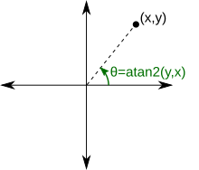
atan2(+0, +0) = +0;

atan2(+0, −0) = +π;  ( 当y是位于y轴正半轴，无限趋近于0的值；x是位于x轴负半轴，无限趋近于0的值，=> 可以看做是在第二象限中位于x轴负半轴的一点 => $\theta夹角为$\pi$）

atan2(−0, +0) = −0;  ( 可以看做是在第四象限中位于x轴正半轴的一点 => $\theta夹角为-0)

atan2(−0, −0) = −π.

用代码验证：

>>> math.atan2(0.0, 0.0) == math.atan2(-0.0, 0.0)
True
>>> math.atan2(0.0, -0.0) == math.atan2(-0.0, -0.0)
False

---

所以，尽管在上面自定义激活函数时，将不可导函数强行加入到pytorch的autograd中运算，数值结果相同；但是注意到-0.0000的出现是程序有bug的提示，严谨考虑仍需要规范定义，如MyReLU。