利用Python学习线性代数 -- 1.1 线性方程组
利用Python学习线性代数 -- 1.1 线性方程组
本节实现的主要功能函数,在源码文件linear_system中,后续章节将作为基本功能调用。
线性方程
线性方程组由一个或多个线性方程组成,如
x_1 - 2 x_2 &= -1\\
-x_1 + 3 x_2 &= 3
\end{array}
\]
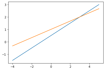
求包含两个变量两个线性方程的方程组的解,等价于求两条直线的交点。
这里可以画出书图1-1和1-2的线性方程组的图形。
通过改变线性方程的参数,观察图形,体会两个方程对应直线平行、相交、重合三种可能。
那么,怎么画二元线性方程的直线呢?
方法是这样的:
假如方程是 \(a x_1 + b x_2 = c\) 的形式,可以写成 \(x_2 = (c - a x_1) / b\)。
在以 \(x_1\) 和\(x_2\)为两个轴的直角坐标系中,\(x_1\)取一组值,如 \((-3, -2.9, -2.8, \dots, 2.9, 3.0)\),
计算相应的 \(x_2\),然后把所有点 \((x_1, x_2)\) 连起来成为一条线。
当 \(b\) 为 \(0\) 时, 则在\(x_1 = c / a\)处画一条垂直线。
# 引入Numpy和 Matplotlib库

import numpy as np

from matplotlib import pyplot as plt
Matplotlib 是Python中使用较多的可视化库,这里只用到了它的一些基本功能。
def draw_line(a, b, c, start=-4,

              stop=5, step=0.01):

    """根据线性方程参数绘制一条直线"""

    # 如果b为0,则画一条垂线

    if np.isclose(b, 0):

        plt.vlines(start, stop, c / a)

    else: # 否则画 y = (c - a*x) / b

        xs = np.arange(start, stop, step)

        plt.plot(xs, (c - a*xs)/b)
# 1.1 图1-1

draw_line(1, -2, -1)

draw_line(-1, 3, 3)

def draw_lines(augmented, start=-4,

              stop=5, step=0.01):

    """给定增广矩阵,画两条线."""

    plt.figure()

    for equation in augmented:

        draw_line(*equation, start, stop, step)

    plt.show()
# Fig. 1-1

# 增广矩阵用二维数组表示

# [[1, -2, -1], [-1, 3, 3]]

# 这些数字对应图1-1对应方程的各项系数

draw_lines([[1, -2, -1], [-1, 3, 3]])
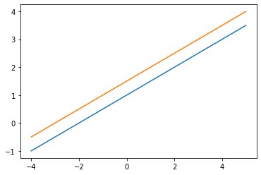
# Fig. 1-2
draw_lines([[1, -2, -2], [-1, 2, 3]])
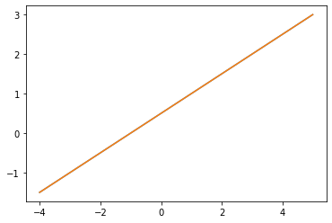
# Fig. 1-3
draw_lines([[1, -2, -1], [-1, 2, 1]])
- 建议:改变这些系数,观察直线,体会两条直线相交、平行和重合的情况
例如
draw_lines([[1, -2, -2], [-1, 2, 9]])
如果对Numpy比较熟悉,则可以采用更简洁的方式实现上述绘图功能。
在计算多条直线方程时,可以利用向量编程的方式,用更少的代码实现。
def draw_lines(augmented, start=-4,

               stop=5, step=0.01):

    """Draw lines represented by augmented matrix on 2-d plane."""

    am = np.asarray(augmented)

    xs = np.arange(start, stop, step).reshape([1, -1])

    # 同时计算两条直线的y值

    ys = (am[:, [-1]] - am[:, [1]]*xs) / am[:, [0]]

    for y in ys:

        plt.plot(xs[0], y)

    plt.show()
矩阵记号
矩阵是一个数表,在程序中通常用二维数组表示,例如
# 嵌套列表表示矩阵

matrix = [[1, -2, 1, 0],

          [0, 2, -8, 8],

          [5, 0, -5, 10]]

matrix
[[1, -2, 1, 0], [0, 2, -8, 8], [5, 0, -5, 10]]
实际工程和研究实践中,往往会采用一些专门的数值计算库,简化和加速计算。
Numpy库是Python中数值计算的常用库。
在Numpy中,多维数组类型称为ndarray,可以理解为n dimensional array。
例如
# Numpy ndarray 表示矩阵

matrix = np.array([[1, -2, 1, 0],

                    [0, 2, -8, 8],

                    [5, 0, -5, 10]])

matrix
array([[ 1, -2,  1,  0],

       [ 0,  2, -8,  8],

       [ 5,  0, -5, 10]])
解线性方程组
本节解线性方程组的方法是 高斯消元法,利用了三种基本行变换。
- 把某个方程换成它与另一个方程的倍数的和;
- 交换两个方程的位置;
- 某个方程的所有项乘以一个非零项。
假设线性方程的增广矩阵是\(A\),其第\(i\)行\(j\)列的元素是\(a_{ij}\)。
消元法的基本步骤是:
- 增广矩阵中有 \(n\) 行,该方法的每一步处理一行。
- 在第\(i\)步,该方法处理第\(i\)行
- 若\(a_{ii}\)为0,则在剩余行 \(\{j| j \in (i, n]\}\)中选择绝对值最大的行\(a_{ij}\)
- 若\(a_{ij}\)为0,返回第1步。
- 否则利用变换2,交换\(A\)的第\(i\)和\(j\)行。
- 若\(a_{ii}\)为0,则在剩余行 \(\{j| j \in (i, n]\}\)中选择绝对值最大的行\(a_{ij}\)
- 利用行变换3,第\(i\)行所有元素除以\(a_{ii}\),使第 \(i\) 个方程的第 \(i\)个 系数为1
- 利用行变换1,\(i\)之后的行减去第\(i\)行的倍数,使这些行的第 \(i\) 列为0
- 在第\(i\)步,该方法处理第\(i\)行
为了理解这些步骤的实现,这里先按书中的例1一步步计算和展示,然后再总结成完整的函数。
例1的增广矩阵是
\begin{array}
&1 & -2 & 1 & 0\\
0 & 2 & -8 & 8\\
5 & 0 & -5 & 10
\end{array}
\right]
\]
# 增广矩阵

A = np.array([[1, -2, 1, 0],

              [0, 2, -8, 8],

              [5, 0, -5, 10]])

# 行号从0开始,处理第0行

i = 0

# 利用变换3,将第i行的 a_ii 转成1。这里a_00已经是1,所不用动

# 然后利用变换1,把第1行第0列,第2行第0列都减成0。

# 这里仅需考虑i列之后的元素,因为i列之前的元素已经是0

#   即第1行减去第0行的0倍

#   而第2行减去第0行的5倍

A[i+1:, i:] = A[i+1:, i:] - A[i+1:, [i]] * A[i, i:]

A
array([[  1,  -2,   1,   0],

       [  0,   2,  -8,   8],

       [  0,  10, -10,  10]])
i = 1

# 利用变换3,将第i行的 a_ii 转成1。

A[i] = A[i] / A[i, i]

A
array([[  1,  -2,   1,   0],

       [  0,   1,  -4,   4],

       [  0,  10, -10,  10]])
# 然后利用变换1,把第2行第i列减成0。

A[i+1:, i:] = A[i+1:, i:] - A[i+1:, [i]] * A[i, i:]

A
array([[  1,  -2,   1,   0],

       [  0,   1,  -4,   4],

       [  0,   0,  30, -30]])
i = 2

# 利用变换3,将第i行的 a_ii 转成1。

A[i] = A[i] / A[i, i]

A
array([[ 1, -2,  1,  0],

       [ 0,  1, -4,  4],

       [ 0,  0,  1, -1]])
消元法的前向过程就结束了,我们可以总结成一个函数
def eliminate_forward(augmented):

    """

    消元法的前向过程.

    返回行阶梯形,以及先导元素的坐标(主元位置)

    """

    A = np.asarray(augmented, dtype=np.float64)

    # row number of the last row

    pivots = []

    i, j = 0, 0

    while i < A.shape[0] and j < A.shape[1]:

        A[i] = A[i] / A[i, j]

        if (i + 1) < A.shape[0]: # 除最后一行外

            A[i+1:, j:] = A[i+1:, j:] - A[i+1:, [j]] * A[i, j:]

        pivots.append((i, j))

        i += 1

        j += 1

    return A, pivots
这里有两个细节值得注意
- 先导元素 \(a_{ij}\),不一定是在主对角线位置,即 \(i\) 不一定等于\(j\).
- 最后一行只需要用变换3把先导元素转为1,没有剩余行需要转换
# 测试一个增广矩阵,例1

A = np.array([[1, -2, 1, 0],

              [0, 2, -8, 8],

              [5, 0, -5, 10]])

A, pivots = eliminate_forward(A)

print(A)

print(pivots)
[[ 1. -2.  1.  0.]

 [ 0.  1. -4.  4.]

 [ 0.  0.  1. -1.]]

[(0, 0), (1, 1), (2, 2)]
消元法的后向过程则更简单一些,对于每一个主元(这里就是前面的\(a_{ii}\)),将其所在的列都用变换1,使其它行对应的列为0.
for i, j in reversed(pivots):

    A[:i, j:] = A[:i, j:] - A[[i], j:] * A[:i, [j]]

A
array([[ 1.,  0.,  0.,  1.],

       [ 0.,  1.,  0.,  0.],

       [ 0.,  0.,  1., -1.]])
def eliminate_backward(simplified, pivots):

    """消元法的后向过程."""

    A = np.asarray(simplified)

    for i, j in reversed(pivots):

        A[:i, j:] = A[:i, j:] - A[[i], j:] * A[:i, [j]]

    return A
至此,结合 eliminate_forward 和eliminate_backward函数,可以解形如例1的线性方程。
然而,存在如例3的线性方程,在eliminate_forward算法进行的某一步,主元为0,需要利用变换2交换两行。
交换行时,可以选择剩余行中,选择当前主元列不为0的任意行,与当前行交换。
这里每次都采用剩余行中,当前主元列绝对值最大的行。
补上行交换的前向过程函数如下
def eliminate_forward(augmented):

    """消元法的前向过程"""

    A = np.asarray(augmented, dtype=np.float64)

    # row number of the last row

    pivots = []

    i, j = 0, 0

    while i < A.shape[0] and j < A.shape[1]:

        # if pivot is zero, exchange rows

        if np.isclose(A[i, j], 0):

            if (i + 1) < A.shape[0]:

                max_k = i + 1 + np.argmax(np.abs(A[i+1:, i]))

            if (i + 1) >= A.shape[0] or np.isclose(A[max_k, i], 0):

                j += 1

                continue

            A[[i, max_k]] = A[[max_k, i]]

        A[i] = A[i] / A[i, j]

        if (i + 1) < A.shape[0]:

            A[i+1:, j:] = A[i+1:, j:] - A[i+1:, [j]] * A[i, j:]

        pivots.append((i, j))

        i += 1

        j += 1

    return A, pivots
行交换时,有一种特殊情况,即剩余所有行的主元列都没有非零元素。
这种情况下,在当前列的右侧寻找不为零的列,作为新的主元列。
# 用例3测试eliminate_forward

aug = [[0, 1, -4, 8],

       [2, -3, 2, 1],

       [4, -8, 12, 1]]

echelon, pivots = eliminate_forward(aug)

print(echelon)

print(pivots)
[[ 1.   -2.    3.    0.25]

 [ 0.    1.   -4.    0.5 ]

 [ 0.    0.    0.    1.  ]]

[(0, 0), (1, 1), (2, 3)]
例3化简的结果与书上略有不同,由行交换策略不同引起,也说明同一个矩阵可能由多个阶梯形。
结合上述的前向和后向过程,即可以给出一个完整的消元法实现
def eliminate(augmented):

    """

    利用消元法前向和后向步骤,化简线性方程组.

    如果是矛盾方程组,则仅输出前向化简结果,并打印提示

    否则输出简化后的方程组,并输出最后一列

    """

    print(np.asarray(augmented))

    A, pivots = eliminate_forward(augmented)

    print(" The echelon form is\n", A)

    print(" The pivots are: ", pivots)

    pivot_cols = {p[1] for p in pivots}

    simplified = eliminate_backward(A, pivots)

    if (A.shape[1]-1) in pivot_cols:

        print(" There is controdictory.\n", simplified)

    elif len(pivots) == (A.shape[1] -1):

        print(" Solution: ", simplified[:, -1])

        is_correct = solution_check(np.asarray(augmented),

                            simplified[:, -1])

        print(" Is the solution correct? ", is_correct)

    else:

        print(" There are free variables.\n", simplified)

    print("-"*30)
eliminate(aug)
[[ 0  1 -4  8]

 [ 2 -3  2  1]

 [ 4 -8 12  1]]

 The echelon form is

 [[ 1.   -2.    3.    0.25]

 [ 0.    1.   -4.    0.5 ]

 [ 0.    0.    0.    1.  ]]

 The pivots are:  [(0, 0), (1, 1), (2, 3)]

 There is controdictory.

 [[ 1.  0. -5.  0.]

 [ 0.  1. -4.  0.]

 [ 0.  0.  0.  1.]]

------------------------------
利用 Sympy 验证消元法实现的正确性
Python的符号计算库Sympy,有化简矩阵为行最简型的方法,可以用来检验本节实现的代码是否正确。
# 导入 sympy的 Matrix模块

from sympy import Matrix
Matrix(aug).rref(simplify=True)

# 返回的是行最简型和主元列的位置
(Matrix([

 [1, 0, -5, 0],

 [0, 1, -4, 0],

 [0, 0,  0, 1]]), (0, 1, 3))
echelon, pivots = eliminate_forward(aug)

simplified = eliminate_backward(echelon, pivots)

print(simplified, pivots)

# 输出与上述rref一致
[[ 1.  0. -5.  0.]

 [ 0.  1. -4.  0.]

 [ 0.  0.  0.  1.]] [(0, 0), (1, 1), (2, 3)]
综合前向和后向步骤,并结果的正确性
综合前向和后向消元,就可以得到完整的消元法过程。
消元结束,如果没有矛盾(最后一列不是主元列),基本变量数与未知数个数一致,则有唯一解,可以验证解是否正确。
验证的方法是将解与系数矩阵相乘,检查与原方程的b列一致。
def solution_check(augmented, solution):

    # 系数矩阵与解相乘

    b = augmented[:, :-1] @ solution.reshape([-1, 1])

    b = b.reshape([-1])

    # 检查乘积向量与b列一致

    return all(np.isclose(b - augmented[:, -1], np.zeros(len(b))))
def eliminate(augmented):

    from sympy import Matrix

    print(np.asarray(augmented))

    A, pivots = eliminate_forward(augmented)

    print(" The echelon form is\n", A)

    print(" The pivots are: ", pivots)

    pivot_cols = {p[1] for p in pivots}

    simplified = eliminate_backward(A, pivots)

    if (A.shape[1]-1) in pivot_cols: # 最后一列是主元列

        print(" There is controdictory.\n", simplified)

    elif len(pivots) == (A.shape[1] -1): # 唯一解

        is_correct = solution_check(np.asarray(augmented),

                            simplified[:, -1])

        print(" Is the solution correct? ", is_correct)

        print(" Solution: \n", simplified)

    else: # 有自由变量

        print(" There are free variables.\n", simplified)

    print("-"*30)

    print("对比Sympy的rref结果")

    print(Matrix(augmented).rref(simplify=True))

    print("-"*30)
测试书中的例子
aug_1_1_1 = [[1, -2, 1, 0],

             [0, 2, -8, 8],

             [5, 0, -5, 10]]

eliminate(aug_1_1_1)

# 1.1 example 3

aug_1_1_3 = [[0, 1, -4, 8],

             [2, -3, 2, 1],

             [4, -8, 12, 1]]

eliminate(aug_1_1_3)

eliminate([[1, -6, 4, 0, -1],

           [0, 2, -7, 0, 4],

           [0, 0, 1, 2, -3],

           [0, 0, 3, 1, 6]])

eliminate([[0, -3, -6, 4, 9],

           [-1, -2, -1, 3, 1],

           [-2, -3, 0, 3, -1],

           [1, 4, 5, -9, -7]])

eliminate([[0, 3, -6, 6, 4, -5],

           [3, -7, 8, -5, 8, 9],

           [3, -9, 12, -9, 6, 15]])
[[ 1 -2  1  0]

 [ 0  2 -8  8]

 [ 5  0 -5 10]]

 The echelon form is

 [[ 1. -2.  1.  0.]

 [ 0.  1. -4.  4.]

 [ 0.  0.  1. -1.]]

 The pivots are:  [(0, 0), (1, 1), (2, 2)]

 Is the solution correct?  True

 Solution:

 [[ 1.  0.  0.  1.]

 [ 0.  1.  0.  0.]

 [ 0.  0.  1. -1.]]

------------------------------

对比Sympy的rref结果

(Matrix([

[1, 0, 0,  1],

[0, 1, 0,  0],

[0, 0, 1, -1]]), (0, 1, 2))

------------------------------

[[ 0  1 -4  8]

 [ 2 -3  2  1]

 [ 4 -8 12  1]]

 The echelon form is

 [[ 1.   -2.    3.    0.25]

 [ 0.    1.   -4.    0.5 ]

 [ 0.    0.    0.    1.  ]]

 The pivots are:  [(0, 0), (1, 1), (2, 3)]

 There is controdictory.

 [[ 1.  0. -5.  0.]

 [ 0.  1. -4.  0.]

 [ 0.  0.  0.  1.]]

------------------------------

对比Sympy的rref结果

(Matrix([

[1, 0, -5, 0],

[0, 1, -4, 0],

[0, 0,  0, 1]]), (0, 1, 3))

------------------------------

[[ 1 -6  4  0 -1]

 [ 0  2 -7  0  4]

 [ 0  0  1  2 -3]

 [ 0  0  3  1  6]]

 The echelon form is

 [[ 1.  -6.   4.   0.  -1. ]

 [ 0.   1.  -3.5  0.   2. ]

 [ 0.   0.   1.   2.  -3. ]

 [-0.  -0.  -0.   1.  -3. ]]

 The pivots are:  [(0, 0), (1, 1), (2, 2), (3, 3)]

 Is the solution correct?  True

 Solution:

 [[ 1.   0.   0.   0.  62. ]

 [ 0.   1.   0.   0.  12.5]

 [ 0.   0.   1.   0.   3. ]

 [-0.  -0.  -0.   1.  -3. ]]

------------------------------

对比Sympy的rref结果

(Matrix([

[1, 0, 0, 0,   62],

[0, 1, 0, 0, 25/2],

[0, 0, 1, 0,    3],

[0, 0, 0, 1,   -3]]), (0, 1, 2, 3))

------------------------------

[[ 0 -3 -6  4  9]

 [-1 -2 -1  3  1]

 [-2 -3  0  3 -1]

 [ 1  4  5 -9 -7]]

 The echelon form is

 [[ 1.   1.5 -0.  -1.5  0.5]

 [-0.   1.   2.  -3.  -3. ]

 [-0.  -0.  -0.   1.  -0. ]

 [ 0.   0.   0.   0.   0. ]]

 The pivots are:  [(0, 0), (1, 1), (2, 3)]

 There are free variables.

 [[ 1.  0. -3.  0.  5.]

 [-0.  1.  2.  0. -3.]

 [-0. -0. -0.  1. -0.]

 [ 0.  0.  0.  0.  0.]]

------------------------------

对比Sympy的rref结果

(Matrix([

[1, 0, -3, 0,  5],

[0, 1,  2, 0, -3],

[0, 0,  0, 1,  0],

[0, 0,  0, 0,  0]]), (0, 1, 3))

------------------------------

[[ 0  3 -6  6  4 -5]

 [ 3 -7  8 -5  8  9]

 [ 3 -9 12 -9  6 15]]

 The echelon form is

 [[ 1.         -2.33333333  2.66666667 -1.66666667  2.66666667  3.        ]

 [ 0.          1.         -2.          2.          1.33333333 -1.66666667]

 [ 0.          0.          0.          0.          1.          4.        ]]

 The pivots are:  [(0, 0), (1, 1), (2, 4)]

 There are free variables.

 [[  1.   0.  -2.   3.   0. -24.]

 [  0.   1.  -2.   2.   0.  -7.]

 [  0.   0.   0.   0.   1.   4.]]

------------------------------

对比Sympy的rref结果

(Matrix([

[1, 0, -2, 3, 0, -24],

[0, 1, -2, 2, 0,  -7],

[0, 0,  0, 0, 1,   4]]), (0, 1, 4))

------------------------------
利用Python学习线性代数 -- 1.1 线性方程组的更多相关文章
- 利用python 学习数据分析 (学习二)
内容学习自: Python for Data Analysis, 2nd Edition 就是这本 纯英文学的很累,对不对取决于百度翻译了 前情提要: 各种方法贴: https://w ...
- 利用python 学习数据分析 (学习四)
内容学习自: Python for Data Analysis, 2nd Edition 就是这本 纯英文学的很累,对不对取决于百度翻译了 前情提要: 各种方法贴: https://w ...
- 利用python 学习数据分析 (学习三)
内容学习自: Python for Data Analysis, 2nd Edition 就是这本 纯英文学的很累,对不对取决于百度翻译了 前情提要: 各种方法贴: https://w ...
- 利用python 学习数据分析 (学习一)
内容学习自: Python for Data Analysis, 2nd Edition 就是这本 纯英文学的很累,对不对取决于百度翻译了 前情提要: 各种方法贴: https://w ...
- 利用python进行数据分析——(一)库的学习
总结一下自己对python常用包:Numpy,Pandas,Matplotlib,Scipy,Scikit-learn 一. Numpy: 标准安装的Python中用列表(list)保存一组值,可以用 ...
- Python 数据分析(二 本实验将学习利用 Python 数据聚合与分组运算,时间序列,金融与经济数据应用等相关知识
Python 数据分析(二) 本实验将学习利用 Python 数据聚合与分组运算,时间序列,金融与经济数据应用等相关知识 第1节 groupby 技术 第2节 数据聚合 第3节 分组级运算和转换 第4 ...
- 利用Python实现一个感知机学习算法
本文主要参考英文教材Python Machine Learning第二章.pdf文档下载链接: https://pan.baidu.com/s/1nuS07Qp 密码: gcb9. 本文主要内容包括利 ...
- 爬虫学习笔记(1)-- 利用Python从网页抓取数据
最近想从一个网站上下载资源,懒得一个个的点击下载了,想写一个爬虫把程序全部下载下来,在这里做一个简单的记录 Python的基础语法在这里就不多做叙述了,黑马程序员上有一个基础的视频教学,可以跟着学习一 ...
- PYTHON学习(三)之利用python进行数据分析(1)---准备工作
学习一门语言就是不断实践,python是目前用于数据分析最流行的语言,我最近买了本书<利用python进行数据分析>(Wes McKinney著),还去图书馆借了本<Python数据 ...
随机推荐
- phpstorm安装步骤是什么?
phpstorm的安装及其激活教程 1.phpstorm安装步骤: (1)下载地址:http://www.jetbrains.com/phpstorm/ 根据自己电脑的32or64位下载,下载完后就是 ...
- postman设置环境变量与全局变量
1.环境变量可以设置多组 设置环境变量 编辑环境变量 2.全局变量只能设置一组 可以在Pre-request Script和Tests中设置全局变量 如:pm.globals.set("na ...
- 21.Nginx代理缓存
1.环境准备 操作系统 应用服务 外网地址 内网地址 CentOS7.6 LB01 10.0.0.5 172.16.1.5 CentOS7.6 Web01 10.0.0.7 172.16.1.7 2. ...
- spring cloud 网关服务
微服务 网关服务 网关服务是微服务体系里面重要的一环. 微服务体系内,各个服务之间都会有通用的功能比如说:鉴权.安全.监控.日志.服务调度转发.这些都是可以单独抽象出来做一个服务来处理.所以微服务网关 ...
- 初级开发者也能码出专业炫酷的3D地图吗?
好看的3D地图搭建出来,一定是要能为开发者所用与业务系统开发中才能真正地体现价值.基因于此,CityBuilder建立了与ThingJS的通道——直转ThingJS代码,支持将配置完成的3D地图一键转 ...
- Nginx 了解一下?
这篇文章主要简单的介绍下 Nginx 的相关知识,主要包括以下几部分内容: Nginx 适用于哪些场景? 为什么会出现 Nginx? Nginx 优点 Nginx 的编译与配置 Nginx 适用于哪些 ...
- Java线程池的正确关闭方法,awaitTermination还不够
问题说明 今天发现了一个问题,颠覆了我之前对关闭线程池的认识. 一直以来,我坚信用shutdown + awaitTermination关闭线程池是最标准的方式. 不过,这次遇到的问题是,子线程用到B ...
- PHP的陷阱
PHP的陷阱 写代码的时候有个疑惑,那就是数组下标不存在的时候就会挂掉Undefined Index XXXX,这是对的,但是有时候他就不报错,这又是矛盾的. 请看下面的例子: $json_raw = ...
- Modbus协议笔记
读线圈:就是说读开关量输出的状态,看看开关量输出的到底是开着的还是关着的,这样说有点不专业,但是好明白.比如要在上位机显示开关量输出的当状态,就得用这个功能码. 写线圈:就是说读开关量输入的状态,开关 ...
- 从函数计算架构看 Serverless 的演进与思考
作者 | 杨皓然 阿里巴巴高级技术专家 导读:云计算之所以能够成为 DT 时代颠覆性力量,是因为其本质是打破传统架构模式.降低成本并简化体系结构,用全新的思维更好的满足了用户需求.而无服务器计算(S ...