Python基础-画图：matplotlib

Python画图主要用到matplotlib这个库。具体来说是pylab和pyplot这两个子库。这两个库可以满足基本的画图需求。

pylab神器：pylab.rcParams.update(params)。这个函数几乎可以调节图的一切属性，包括但不限于：坐标范围，axes标签字号大小，xtick,ytick标签字号，图线宽，legend字号等。

具体参数参看官方文档：http://matplotlib.org/users/customizing.html

---

scatter和 plot 函数的不同之处

scatter才是离散点的绘制程序，plot准确来说是绘制线图的，当然也可以画离散点。

scatter/scatter3做散点的能力更强，因为他可以对散点进行单独设置
所以消耗也比plot/plot3大
所以如果每个散点都是一致的时候，还是用plot/plot3好以下
如果要做一些plot没法完成的事情那就只能用scatter了

scatter强大，但是较慢。所以如果你只是做实例中的图，plot足够了。

---

 plt.ion()用于连续显示。

# plot the real data
fig = plt.figure()
ax = fig.add_subplot(1,1,1)
ax.scatter(x_data, y_data)
plt.ion()#本次运行请注释，全局运行不要注释
plt.show()

---

首先在python中使用任何第三方库时，都必须先将其引入。即：

import matplotlib.pyplot as plt

• 1

或者：

from matplotlib.pyplot import *

1.建立空白图

fig = plt.figure()

也可以指定所建立图的大小

fig = plt.figure(figsize=(4,2))

也可以建立一个包含多个子图的图，使用语句：

plt.figure(figsize=(12,6))
plt.subplot(231)
plt.subplot(232)
plt.subplot(233)
plt.subplot(234)
plt.subplot(235)
plt.subplot(236)
plt.show()

其中subplot()函数中的三个数字，第一个表示Y轴方向的子图个数，第二个表示X轴方向的子图个数，第三个则表示当前要画图的焦点。

当然上述写法并不是唯一的，比如我们也可以这样写：

fig = plt.figure(figsize=(6, 6))
ax1 = fig.add_subplot(221)
ax2 = fig.add_subplot(222)
ax3 = fig.add_subplot(223)
ax4 = fig.add_subplot(224)
plt.show()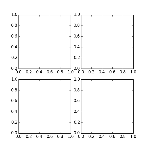

plt.subplot(111)和plt.subplot(1,1,1)是等价的。意思是将区域分成1行1列，当前画的是第一个图（排序由行至列）。

plt.subplot(211)意思就是将区域分成2行1列，当前画的是第一个图（第一行，第一列）。以此类推，只要不超过10，逗号就可省去。

可以看到图中的x,y轴坐标都是从0到1，当然有时候我们需要其他的坐标起始值。 
此时可以使用语句指定：

ax1.axis([-1, 1, -1, 1])

或者：

plt.axis([-1, 1, -1, 1])

效果如下：

2.向空白图中添加内容，想你所想，画你所想

首先给出一组数据：

x = [1, 2, 3, 4, 5]
y = [2.3, 3.4, 1.2, 6.6, 7.0]

A.画散点图*

plt.scatter(x, y, color='r', marker='+')
plt.show()

效果如下：

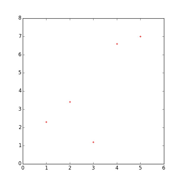
这里的参数意义：

1. x为横坐标向量，y为纵坐标向量，x,y的长度必须一致。

2. 控制颜色：color为散点的颜色标志，常用color的表示如下：

   b---blue   c---cyan  g---green    k----black
   m---magenta r---red  w---white    y----yellow

   有四种表示颜色的方式:

   • 用全名
   • 16进制，如：#FF00FF
   • 灰度强度，如：‘0.7’

3. 控制标记风格：marker为散点的标记，标记风格有多种：

   .  Point marker
   ,  Pixel marker
   o  Circle marker
   v  Triangle down marker
   ^  Triangle up marker
   <  Triangle left marker
   >  Triangle right marker
   1  Tripod down marker
   2  Tripod up marker
   3  Tripod left marker
   4  Tripod right marker
   s  Square marker
   p  Pentagon marker
   *  Star marker
   h  Hexagon marker
   H  Rotated hexagon D Diamond marker
   d  Thin diamond marker
   | Vertical line (vlinesymbol) marker
   _  Horizontal line (hline symbol) marker
   +  Plus marker
   x  Cross (x) marker

B.函数图（折线图）

数据还是上面的。

fig = plt.figure(figsize=(12, 6))
plt.subplot(121)
plt.plot(x, y, color='r', linestyle='-')
plt.subplot(122)
plt.plot(x, y, color='r', linestyle='--')
plt.show()

效果如下：

这里有一个新的参数linestyle，控制的是线型的格式：符号和线型之间的对应关系

-      实线
--     短线
-.     短点相间线
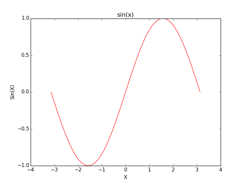
：     虚点线

另外除了给出数据画图之外，我们也可以利用函数表达式进行画图，例如：y=sin(x)

from math import *
from numpy import *
x = arange(-math.pi, math.pi, 0.01)
y = [sin(xx) for xx in x]
plt.figure()
plt.plot(x, y, color='r', linestyle='-.')
plt.show()

效果如下：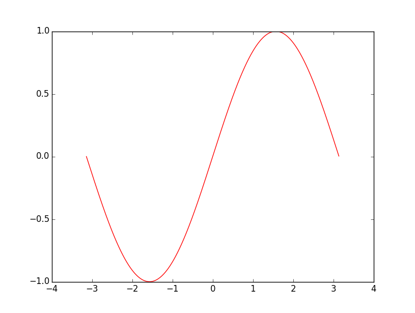

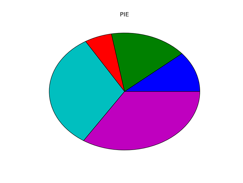
C.扇形图

示例：

import matplotlib.pyplot as plt
y = [2.3, 3.4, 1.2, 6.6, 7.0]
plt.figure()
plt.pie(y)
plt.title('PIE')
plt.show()

效果如下：

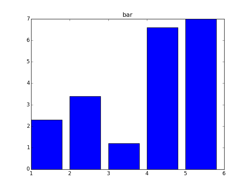
D.柱状图bar

示例：

import matplotlib.pyplot as plt
x = [1, 2, 3, 4, 5]
y = [2.3, 3.4, 1.2, 6.6, 7.0]

plt.figure()
plt.bar(x, y)
plt.title("bar")
plt.show()

效果如下：

E.二维图形（等高线，本地图片等）

import matplotlib.pyplot as plt
import numpy as np
import matplotlib.image as mpimg
# 2D data

delta = 0.025
x = y = np.arange(-3.0, 3.0, delta)
X, Y = np.meshgrid(x, y)
Z = Y**2 + X**2
plt.figure(figsize=(12, 6))
plt.subplot(121)
plt.contour(X, Y, Z)
plt.colorbar()
plt.title("contour")

# read image

img=mpimg.imread('marvin.jpg')

plt.subplot(122)
plt.imshow(img)
plt.title("imshow")
plt.show()
#plt.savefig("matplot_sample.jpg")

效果图：

F.对所画图进行补充

__author__ = 'wenbaoli'

import matplotlib.pyplot as plt
from math import *
from numpy import *
x = arange(-math.pi, math.pi, 0.01)
y = [sin(xx) for xx in x]
plt.figure()
plt.plot(x, y, color='r', linestyle='-')
plt.xlabel(u'X')#fill the meaning of X axis
plt.ylabel(u'Sin(X)')#fill the meaning of Y axis
plt.title(u'sin(x)')#add the title of the figure

plt.show()

效果图： 

画网络图，要用到networkx这个库，下面给出一个实例：

import networkx as nx import pylab as plt g = nx.Graph() g.add_edge(1,2,weight = 4) g.add_edge(1,3,weight = 7) g.add_edge(1,4,weight = 8) g.add_edge(1,5,weight = 3) g.add_edge(1,9,weight = 3)   g.add_edge(1,6,weight = 6) g.add_edge(6,7,weight = 7) g.add_edge(6,8,weight = 7)    g.add_edge(6,9,weight = 6) g.add_edge(9,10,weight = 7) g.add_edge(9,11,weight = 6)       fixed_pos = {1:(1,1),2:(0.7,2.2),3:(0,1.8),4:(1.6,2.3),5:(2,0.8),6:(-0.6,-0.6),7:(-1.3,0.8), 8:(-1.5,-1), 9:(0.5,-1.5), 10:(1.7,-0.8), 11:(1.5,-2.3)} #set fixed layout location       #pos=nx.spring_layout(g) # or you can use other layout set in the module nx.draw_networkx_nodes(g,pos = fixed_pos,nodelist=[1,2,3,4,5], node_color = 'g',node_size = 600) nx.draw_networkx_edges(g,pos = fixed_pos,edgelist=[(1,2),(1,3),(1,4),(1,5),(1,9)],edge_color='g',width = [4.0,4.0,4.0,4.0,4.0],label = [1,2,3,4,5],node_size = 600)     nx.draw_networkx_nodes(g,pos = fixed_pos,nodelist=[6,7,8], node_color = 'r',node_size = 600) nx.draw_networkx_edges(g,pos = fixed_pos,edgelist=[(6,7),(6,8),(1,6)],width = [4.0,4.0,4.0],edge_color='r',node_size = 600)   nx.draw_networkx_nodes(g,pos = fixed_pos,nodelist=[9,10,11], node_color = 'b',node_size = 600) nx.draw_networkx_edges(g,pos = fixed_pos,edgelist=[(6,9),(9,10),(9,11)],width = [4.0,4.0,4.0],edge_color='b',node_size = 600)     plt.text(fixed_pos[1][0],fixed_pos[1][1]+0.2, s = '1',fontsize = 40) plt.text(fixed_pos[2][0],fixed_pos[2][1]+0.2, s = '2',fontsize = 40) plt.text(fixed_pos[3][0],fixed_pos[3][1]+0.2, s = '3',fontsize = 40) plt.text(fixed_pos[4][0],fixed_pos[4][1]+0.2, s = '4',fontsize = 40) plt.text(fixed_pos[5][0],fixed_pos[5][1]+0.2, s = '5',fontsize = 40) plt.text(fixed_pos[6][0],fixed_pos[6][1]+0.2, s = '6',fontsize = 40) plt.text(fixed_pos[7][0],fixed_pos[7][1]+0.2, s = '7',fontsize = 40) plt.text(fixed_pos[8][0],fixed_pos[8][1]+0.2, s = '8',fontsize = 40) plt.text(fixed_pos[9][0],fixed_pos[9][1]+0.2, s = '9',fontsize = 40) plt.text(fixed_pos[10][0],fixed_pos[10][1]+0.2, s = '10',fontsize = 40) plt.text(fixed_pos[11][0],fixed_pos[11][1]+0.2, s = '11',fontsize = 40)       plt.show()

结果如下：