CS231n 2016 通关 第五、六章 Fully-Connected Neural Nets 作业
要求:实现任意层数的NN。
每一层结构包含:


1、前向传播和反向传播函数;2、每一层计算的相关数值
cell 1 依旧是显示的初始设置
 # As usual, a bit of setup

 import time

 import numpy as np

 import matplotlib.pyplot as plt

 from cs231n.classifiers.fc_net import *

 from cs231n.data_utils import get_CIFAR10_data

 from cs231n.gradient_check import eval_numerical_gradient, eval_numerical_gradient_array

 from cs231n.solver import Solver

 %matplotlib inline

 plt.rcParams['figure.figsize'] = (10.0, 8.0) # set default size of plots

 plt.rcParams['image.interpolation'] = 'nearest'

 plt.rcParams['image.cmap'] = 'gray'

 # for auto-reloading external modules

 # see http://stackoverflow.com/questions/1907993/autoreload-of-modules-in-ipython

 %load_ext autoreload

 %autoreload 2

 def rel_error(x, y):

   """ returns relative error """

   return np.max(np.abs(x - y) / (np.maximum(1e-8, np.abs(x) + np.abs(y))))
cell 2 读取cifar数据,并显示维度信息
 # Load the (preprocessed) CIFAR10 data.

 data = get_CIFAR10_data()

 for k, v in data.iteritems():

   print '%s: ' % k, v.shape
cell 3 使用随机生成的数据,测试affine 前向传播函数
 # Test the affine_forward function

 num_inputs = 2

 input_shape = (4, 5, 6)

 output_dim = 3

 input_size = num_inputs * np.prod(input_shape)

 # input_size        240

 weight_size = output_dim * np.prod(input_shape)

 # iweight_size   360

 x = np.linspace(-0.1, 0.5, num=input_size).reshape(num_inputs, *input_shape)

 #(2,4,5,6)     -1->0.5

 w = np.linspace(-0.2, 0.3, num=weight_size).reshape(np.prod(input_shape), output_dim)

 #(120, 3)     -0.2->0.3

 b = np.linspace(-0.3, 0.1, num=output_dim)

 #(3,)             0.3->0.1

 #2  num_inputs  120 input_shape 2*120  * 120*3 >>2*3

 out, _ = affine_forward(x, w, b)

 correct_out = np.array([[ 1.49834967,  1.70660132,  1.91485297],

                         [ 3.25553199,  3.5141327,   3.77273342]])

 # Compare your output with ours. The error should be around 1e-9.

 print 'Testing affine_forward function:'

 print 'difference: ', rel_error(out, correct_out)
结果:
 affine_forward(x, w, b)函数内容
 def affine_forward(x, w, b):

   """

   Computes the forward pass for an affine (fully-connected) layer.

   The input x has shape (N, d_1, ..., d_k) and contains a minibatch of N

   examples, where each example x[i] has shape (d_1, ..., d_k). We will

   reshape each input into a vector of dimension D = d_1 * ... * d_k, and

   then transform it to an output vector of dimension M.

   Inputs:

   - x: A numpy array containing input data, of shape (N, d_1, ..., d_k)

   - w: A numpy array of weights, of shape (D, M)

   - b: A numpy array of biases, of shape (M,)

   Returns a tuple of:

   - out: output, of shape (N, M)

   - cache: (x, w, b)

   """

   out = None

   #############################################################################

   # TODO: Implement the affine forward pass. Store the result in out. You     #

   # will need to reshape the input into rows.                                 #

   #############################################################################

   N = x.shape[0]

   D = x.size / N

   x = x.reshape(N, D)

   #2  num_inputs  120 input_shape 2*120  * 120*3 >>2*3

   out = np.dot(x,w) + b

   #############################################################################

   #                             END OF YOUR CODE                              #

   #############################################################################

   cache = (x, w, b)

   return out, cache
cell 4 反向传播,计算梯度是否正确
 # Test the affine_backward function

 x = np.random.randn(10, 2, 3)

 w = np.random.randn(6, 5)

 b = np.random.randn(5)

 dout = np.random.randn(10, 5)

 #x (10,2,3)      w (6,5)       b 5       dout (10,5)

 dx_num = eval_numerical_gradient_array(lambda x: affine_forward(x, w, b)[0], x, dout)

 dw_num = eval_numerical_gradient_array(lambda w: affine_forward(x, w, b)[0], w, dout)

 db_num = eval_numerical_gradient_array(lambda b: affine_forward(x, w, b)[0], b, dout)

 _, cache = affine_forward(x, w, b)

 #g = lambda i : range(i)

 #print g(len(cache))

 #for i in range (len(cache)):

 #  print  cache[i].shape

 #(10, 6)

 #(6, 5)

 #(5,)

 dx, dw, db = affine_backward(dout, cache)

 print dx.shape

 dx = dx.reshape(10, 2, 3)

 # The error should be around 1e-10

 print 'Testing affine_backward function:'

 print 'dx error: ', rel_error(dx_num, dx)

 print 'dw error: ', rel_error(dw_num, dw)

 print 'db error: ', rel_error(db_num, db)
结果:

affine_backward(dout, cache)内容:
 def affine_backward(dout, cache):

   """

   Computes the backward pass for an affine layer.

   Inputs:

   - dout: Upstream derivative, of shape (N, M)

   - cache: Tuple of:

     - x: Input data, of shape (N, d_1, ... d_k)

     - w: Weights, of shape (D, M)

   Returns a tuple of:

   - dx: Gradient with respect to x, of shape (N, d1, ..., d_k)

   - dw: Gradient with respect to w, of shape (D, M)

   - db: Gradient with respect to b, of shape (M,)

   """

   x, w, b = cache

   dx, dw, db = None, None, None

   #(10, 6)

   #(6, 5)

   #(5,)

   #############################################################################

   # TODO: Implement the affine backward pass.                                 #

   #############################################################################

   #loss   ==>>dout 10 *5

   #dx    ==>> 10*5 *  5*6 >>>10*6

   dx = np.dot(dout,w.T)

   #dw   ==>>6*10 * 10*5 >>>6*5

   dw = np.dot(x.T,dout)

   # db  ==>> 5

   db = np.sum(dout,axis=0)

   #############################################################################

   #                             END OF YOUR CODE                              #

   #############################################################################

   return dx, dw, db
cell 5 ReLU 的前向传播
 # Test the relu_forward function

 x = np.linspace(-0.5, 0.5, num=12).reshape(3, 4)

 out, _ = relu_forward(x)

 correct_out = np.array([[ 0.,          0.,          0.,          0.,        ],

                         [ 0.,          0.,          0.04545455,  0.13636364,],

                         [ 0.22727273,  0.31818182,  0.40909091,  0.5,       ]])

 # Compare your output with ours. The error should be around 1e-8

 print 'Testing relu_forward function:'

 print 'difference: ', rel_error(out, correct_out)
结果:

relu_forward(x)内容:
 def relu_forward(x):

   """

   Computes the forward pass for a layer of rectified linear units (ReLUs).

   Input:

   - x: Inputs, of any shape

   Returns a tuple of:

   - out: Output, of the same shape as x

   - cache: x

   """

   out = None

   #############################################################################

   # TODO: Implement the ReLU forward pass.                                    #

   #############################################################################

   out = x*(x>0)

   #############################################################################

   #                             END OF YOUR CODE                              #

   #############################################################################

   cache = x

   return out, cache
cell 6 ReLU 反向传播
 x = np.random.randn(10, 10)

 dout = np.random.randn(*x.shape)

 dx_num = eval_numerical_gradient_array(lambda x: relu_forward(x)[0], x, dout)

 _, cache = relu_forward(x)

 dx = relu_backward(dout, cache)

 # The error should be around 1e-12

 print 'Testing relu_backward function:'

 print 'dx error: ', rel_error(dx_num, dx)
结果:

relu_forward(x)内容:
 def relu_backward(dout, cache):

   """

   Computes the backward pass for a layer of rectified linear units (ReLUs).

   Input:

   - dout: Upstream derivatives, of any shape

   - cache: Input x, of same shape as dout

   Returns:

   - dx: Gradient with respect to x

   """

   dx, x = None, cache

   #############################################################################

   # TODO: Implement the ReLU backward pass.                                   #

   #############################################################################

   dx = dout * (x>=0)

   #############################################################################

   #                             END OF YOUR CODE                              #

   #############################################################################

   return dx
cell 7 affine + ReLU 组合:
 from cs231n.layer_utils import affine_relu_forward, affine_relu_backward

 x = np.random.randn(2, 3, 4)

 w = np.random.randn(12, 10)

 b = np.random.randn(10)

 dout = np.random.randn(2, 10)

 out, cache = affine_relu_forward(x, w, b)

 dx, dw, db = affine_relu_backward(dout, cache)

 dx_num = eval_numerical_gradient_array(lambda x: affine_relu_forward(x, w, b)[0], x, dout)

 dw_num = eval_numerical_gradient_array(lambda w: affine_relu_forward(x, w, b)[0], w, dout)

 db_num = eval_numerical_gradient_array(lambda b: affine_relu_forward(x, w, b)[0], b, dout)

 dx = dx.reshape(2, 3, 4)

 print 'Testing affine_relu_forward:'

 print 'dx error: ', rel_error(dx_num, dx)

 print 'dw error: ', rel_error(dw_num, dw)

 print 'db error: ', rel_error(db_num, db)
结果:

affine_relu_forward(x, w, b):
 def affine_relu_forward(x, w, b):

   """

   Convenience layer that perorms an affine transform followed by a ReLU

   Inputs:

   - x: Input to the affine layer

   - w, b: Weights for the affine layer

   Returns a tuple of:

   - out: Output from the ReLU

   - cache: Object to give to the backward pass

   """

   a, fc_cache = affine_forward(x, w, b)

   out, relu_cache = relu_forward(a)

   cache = (fc_cache, relu_cache)

   return out, cache
affine_relu_backward(dout, cache):
 def affine_relu_backward(dout, cache):

   """

   Backward pass for the affine-relu convenience layer

   """

   fc_cache, relu_cache = cache

   da = relu_backward(dout, relu_cache)

   dx, dw, db = affine_backward(da, fc_cache)

   return dx, dw, db
cell 8 Softmax SVM
这两层的代码在之前已经实现过。并且原文件也给出了。这里不再解释。原理同上。
cell 9 Two-layer network
实现: The architecure should be affine - relu - affine - softmax.
原理依旧是链式法则。
先前向传播,记录传播中用到的数值,之后的偏导需要用到,然后反向传播。
N, D, H, C = 3, 5, 50, 7
X = np.random.randn(N, D)
y = np.random.randint(C, size=N) std = 1e-2
model = TwoLayerNet(input_dim=D, hidden_dim=H, num_classes=C, weight_scale=std)
# 3 example 5 input 50 hidden 7 class
#w1 5*50 b1 50 w2 50*7 b2 7
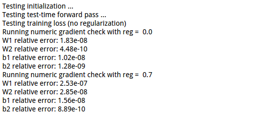
print 'Testing initialization ... '
W1_std = abs(model.params['W1'].std() - std)
b1 = model.params['b1']
W2_std = abs(model.params['W2'].std() - std)
b2 = model.params['b2']
assert W1_std < std / 10, 'First layer weights do not seem right'
assert np.all(b1 == 0), 'First layer biases do not seem right'
assert W2_std < std / 10, 'Second layer weights do not seem right'
assert np.all(b2 == 0), 'Second layer biases do not seem right' print 'Testing test-time forward pass ... '
model.params['W1'] = np.linspace(-0.7, 0.3, num=D*H).reshape(D, H)
model.params['b1'] = np.linspace(-0.1, 0.9, num=H)
model.params['W2'] = np.linspace(-0.3, 0.4, num=H*C).reshape(H, C)
model.params['b2'] = np.linspace(-0.9, 0.1, num=C)
X = np.linspace(-5.5, 4.5, num=N*D).reshape(D, N).T
scores = model.loss(X)
correct_scores = np.asarray(
[[11.53165108, 12.2917344, 13.05181771, 13.81190102, 14.57198434, 15.33206765, 16.09215096],
[12.05769098, 12.74614105, 13.43459113, 14.1230412, 14.81149128, 15.49994135, 16.18839143],
[12.58373087, 13.20054771, 13.81736455, 14.43418138, 15.05099822, 15.66781506, 16.2846319 ]])
scores_diff = np.abs(scores - correct_scores).sum()
assert scores_diff < 1e-6, 'Problem with test-time forward pass' print 'Testing training loss (no regularization)'
y = np.asarray([0, 5, 1])
loss, grads = model.loss(X, y)
correct_loss = 3.4702243556
assert abs(loss - correct_loss) < 1e-10, 'Problem with training-time loss' model.reg = 1.0
loss, grads = model.loss(X, y)
correct_loss = 26.5948426952
assert abs(loss - correct_loss) < 1e-10, 'Problem with regularization loss' for reg in [0.0, 0.7]:
print 'Running numeric gradient check with reg = ', reg
model.reg = reg
loss, grads = model.loss(X, y) for name in sorted(grads):
f = lambda _: model.loss(X, y)[0]
grad_num = eval_numerical_gradient(f, model.params[name], verbose=False)
print '%s relative error: %.2e' % (name, rel_error(grad_num, grads[name]))
结果:
涉及的TwoLayerNet 类:
 class TwoLayerNet(object):

     """

     A two-layer fully-connected neural network with ReLU nonlinearity and

     softmax loss that uses a modular layer design. We assume an input dimension

     of D, a hidden dimension of H, and perform classification over C classes.

     The architecure should be affine - relu - affine - softmax.

     Note that this class does not implement gradient descent; instead, it

     will interact with a separate Solver object that is responsible for running

     optimization.

     The learnable parameters of the model are stored in the dictionary

     self.params that maps parameter names to numpy arrays.

     """

     def __init__(self, input_dim=3 * 32 * 32, hidden_dim=100, num_classes=10,

                  weight_scale=1e-3, reg=0.0):

         """

         Initialize a new network.

         Inputs:

         - input_dim: An integer giving the size of the input

         - hidden_dim: An integer giving the size of the hidden layer

         - num_classes: An integer giving the number of classes to classify

         - dropout: Scalar between 0 and 1 giving dropout strength.

         - weight_scale: Scalar giving the standard deviation for random

           initialization of the weights.

         - reg: Scalar giving L2 regularization strength.

         """

         self.params = {}

         self.reg = reg

         self.D = input_dim

         self.M = hidden_dim

         self.C = num_classes

         self.reg = reg

         w1 = weight_scale * np.random.randn(self.D, self.M)

         b1 = np.zeros(hidden_dim)

         w2 = weight_scale * np.random.randn(self.M, self.C)

         b2 = np.zeros(self.C)

         self.params.update({'W1': w1,

                             'W2': w2,

                             'b1': b1,

                             'b2': b2})

     def loss(self, X, y=None):

         """

         Compute loss and gradient for a minibatch of data.

         Inputs:

         - X: Array of input data of shape (N, d_1, ..., d_k)

         - y: Array of labels, of shape (N,). y[i] gives the label for X[i].

         Returns:

         If y is None, then run a test-time forward pass of the model and return:

         - scores: Array of shape (N, C) giving classification scores, where

           scores[i, c] is the classification score for X[i] and class c.

         If y is not None, then run a training-time forward and backward pass and

         return a tuple of:

         - loss: Scalar value giving the loss

         - grads: Dictionary with the same keys as self.params, mapping parameter

           names to gradients of the loss with respect to those parameters.

         """

         #######################################################################

         # TODO: Implement the backward pass for the two-layer net. Store the loss  #

         # in the loss variable and gradients in the grads dictionary. Compute data #

         # loss using softmax, and make sure that grads[k] holds the gradients for  #

         # self.params[k]. Don't forget to add L2 regularization!                   #

         #                                                                          #

         # NOTE: To ensure that your implementation matches ours and you pass the   #

         # automated tests, make sure that your L2 regularization includes a factor #

         # of 0.5 to simplify the expression for the gradient.                      #

         #######################################################################

         W1, b1, W2, b2 = self.params['W1'], self.params[

             'b1'], self.params['W2'], self.params['b2']

         X = X.reshape(X.shape[0], self.D)

         # Forward into first layer

         hidden_layer, cache_hidden_layer = affine_relu_forward(X, W1, b1)

         # Forward into second layer

         scores, cache_scores = affine_forward(hidden_layer, W2, b2)

         # If y is None then we are in test mode so just return scores

         if y is None:

             return scores

         data_loss, dscores = softmax_loss(scores, y)

         reg_loss = 0.5 * self.reg * np.sum(W1**2)

         reg_loss += 0.5 * self.reg * np.sum(W2**2)

         loss = data_loss + reg_loss

         # Backpropagaton

         grads = {}

         # Backprop into second layer

         dx1, dW2, db2 = affine_backward(dscores, cache_scores)

         dW2 += self.reg * W2

         # Backprop into first layer

         dx, dW1, db1 = affine_relu_backward(

             dx1, cache_hidden_layer)

         dW1 += self.reg * W1

         grads.update({'W1': dW1,

                       'b1': db1,

                       'W2': dW2,

                       'b2': db2})

         return loss, grads
cell 10 使用独立的solver对模型进行训练。
之前训练函数是包含在模型类的方法中的。这样可以对参数》》batch size 正则衰减等值进行修改。
使用独立的solver进行训练,逻辑更清晰。
得到的结果用图像显示:

cell 13 建立隐藏层可选的模型
 N, D, H1, H2, C = 2, 15, 20, 30, 10

 X = np.random.randn(N, D)

 y = np.random.randint(C, size=(N,))

 for reg in [0, 3.14]:

   print 'Running check with reg = ', reg

   model = FullyConnectedNet([H1, H2], input_dim=D, num_classes=C,

                             reg=reg, weight_scale=5e-2, dtype=np.float64)

   loss, grads = model.loss(X, y)

   print 'Initial loss: ', loss

   for name in sorted(grads):

     f = lambda _: model.loss(X, y)[0]

     grad_num = eval_numerical_gradient(f, model.params[name], verbose=False, h=1e-5)

     print '%s relative error: %.2e' % (name, rel_error(grad_num, grads[name]))
由于其中的FullyConnectedNet类包含的内容较多,不在这里贴了。
主要步骤:
对于不同的层数,建立对应的参数:
         Ws = {'W' + str(i + 1):

               weight_scale * np.random.randn(dims[i], dims[i + 1]) for i in range(len(dims) - 1)}

         b = {'b' + str(i + 1): np.zeros(dims[i + 1])

              for i in range(len(dims) - 1)}
之后便是使用这些参数,原理是一致的。
cell 16 SGD+Momentum
 def sgd_momentum(w, dw, config=None):

   """

   Performs stochastic gradient descent with momentum.

   config format:

   - learning_rate: Scalar learning rate.

   - momentum: Scalar between 0 and 1 giving the momentum value.

     Setting momentum = 0 reduces to sgd.

   - velocity: A numpy array of the same shape as w and dw used to store a moving

     average of the gradients.

   """

   if config is None: config = {}

   config.setdefault('learning_rate', 1e-2)

   config.setdefault('momentum', 0.9)

   v = config.get('velocity', np.zeros_like(w))

   next_w = None

   #############################################################################

   # TODO: Implement the momentum update formula. Store the updated value in   #

   # the next_w variable. You should also use and update the velocity v.       #

   #############################################################################

   v = config['momentum']*v - config['learning_rate']*dw

   next_w = v+w

   #############################################################################

   #                             END OF YOUR CODE                              #

   #############################################################################

   config['velocity'] = v

   return next_w, config
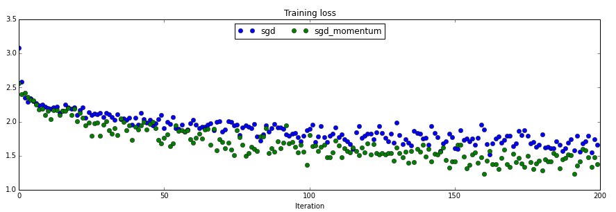
相比较而言,sgd_momentum 收敛的速度更快。
cell 18 rmsprop
 def rmsprop(x, dx, config=None):

   """

   Uses the RMSProp update rule, which uses a moving average of squared gradient

   values to set adaptive per-parameter learning rates.

   config format:

   - learning_rate: Scalar learning rate.

   - decay_rate: Scalar between 0 and 1 giving the decay rate for the squared

     gradient cache.

   - epsilon: Small scalar used for smoothing to avoid dividing by zero.

   - cache: Moving average of second moments of gradients.

   """

   if config is None: config = {}

   config.setdefault('learning_rate', 1e-2)

   config.setdefault('decay_rate', 0.99)

   config.setdefault('epsilon', 1e-8)

   config.setdefault('cache', np.zeros_like(x))

   next_x = None

   #############################################################################

   # TODO: Implement the RMSprop update formula, storing the next value of x   #

   # in the next_x variable. Don't forget to update cache value stored in      #

   # config['cache'].                                                          #

   #############################################################################

   config['cache'] = config['decay_rate']*config['cache'] + (1 - config['decay_rate'])*dx**2

   next_x = x - config['learning_rate']*dx / (np.sqrt(config['cache']) + config['epsilon'])

   #############################################################################

   #                             END OF YOUR CODE                              #

   #############################################################################

   return next_x, config
cell 19 adam
 def adam(x, dx, config=None):

   """

   Uses the Adam update rule, which incorporates moving averages of both the

   gradient and its square and a bias correction term.

   config format:

   - learning_rate: Scalar learning rate.

   - beta1: Decay rate for moving average of first moment of gradient.

   - beta2: Decay rate for moving average of second moment of gradient.

   - epsilon: Small scalar used for smoothing to avoid dividing by zero.

   - m: Moving average of gradient.

   - v: Moving average of squared gradient.

   - t: Iteration number.

   """

   if config is None: config = {}

   config.setdefault('learning_rate', 1e-3)

   config.setdefault('beta1', 0.9)

   config.setdefault('beta2', 0.999)

   config.setdefault('epsilon', 1e-8)

   config.setdefault('m', np.zeros_like(x))

   config.setdefault('v', np.zeros_like(x))

   config.setdefault('t', 1e5)

   next_x = None

   beta_1 = config['beta1']

   beta_2 = config['beta2']

   #############################################################################

   # TODO: Implement the Adam update formula, storing the next value of x in   #

   # the next_x variable. Don't forget to update the m, v, and t variables     #

   # stored in config.                                                         #

   #############################################################################

   config['t'] = config['t'] + 1

   config['m'] = config['m'] * config['beta1'] + (1 - config['beta1']) * dx

   config['v'] = config['v'] * config['beta2'] + (1 - config['beta2']) * (dx ** 2)

   beta_1 = 1 - (beta_1**config['t'])

   beta_2 = np.sqrt(1 - (beta_2**config['t']))

   config['learning_rate'] = config['learning_rate'] * (beta_2/beta_1)

   next_x = x - ((config['learning_rate'] * config['m']) / (np.sqrt(config['v']+config['epsilon'])))

   #############################################################################

   #                             END OF YOUR CODE                              #

   #############################################################################

   return next_x, config
4中方法的收敛速度比较:
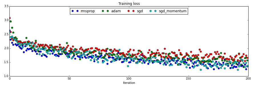
最终会给出所有的代码。
附:通关CS231n企鹅群:578975100 validation:DL-CS231n
CS231n 2016 通关 第五、六章 Fully-Connected Neural Nets 作业的更多相关文章
- CS231n 2016 通关 第五、六章 Dropout 作业
Dropout的作用: cell 1 - cell 2 依旧 cell 3 Dropout层的前向传播 核心代码: train 时: if mode == 'train': ############ ...
- CS231n 2016 通关 第五、六章 Batch Normalization 作业
BN层在实际中应用广泛. 上一次总结了使得训练变得简单的方法,比如SGD+momentum RMSProp Adam,BN是另外的方法. cell 1 依旧是初始化设置 cell 2 读取cifar- ...
- CS231n 2016 通关 第五章 Training NN Part1
在上一次总结中,总结了NN的基本结构. 接下来的几次课,对一些具体细节进行讲解. 比如激活函数.参数初始化.参数更新等等. ====================================== ...
- CS231n 2016 通关 第四章-NN 作业
cell 1 显示设置初始化 # A bit of setup import numpy as np import matplotlib.pyplot as plt from cs231n.class ...
- CS231n 2016 通关 第六章 Training NN Part2
本章节讲解 参数更新 dropout ================================================================================= ...
- CS231n 2016 通关 第三章-SVM与Softmax
1===本节课对应视频内容的第三讲,对应PPT是Lecture3 2===本节课的收获 ===熟悉SVM及其多分类问题 ===熟悉softmax分类问题 ===了解优化思想 由上节课即KNN的分析步骤 ...
- CS231n 2016 通关 第四章-反向传播与神经网络(第一部分)
在上次的分享中,介绍了模型建立与使用梯度下降法优化参数.梯度校验,以及一些超参数的经验. 本节课的主要内容: 1==链式法则 2==深度学习框架中链式法则 3==全连接神经网络 =========== ...
- CS231n 2016 通关 第三章-Softmax 作业
在完成SVM作业的基础上,Softmax的作业相对比较轻松. 完成本作业需要熟悉与掌握的知识: cell 1 设置绘图默认参数 mport random import numpy as np from ...
- CS231n 2016 通关 第三章-SVM 作业分析
作业内容,完成作业便可熟悉如下内容: cell 1 设置绘图默认参数 # Run some setup code for this notebook. import random import nu ...
随机推荐
- vue2.0 + vux (三)MySettings 页
1.MySettings.vue <!-- 我的设置 --> <template> <div> <img class="img_1" sr ...
- 可在 html5 游戏中使用的 js 工具库
可在 html5 游戏中使用的 js 工具库 作者: 木頭 时间: September 21, 2014 分类: Utilities,Game 使用 cocos2d-js 3.0 开发游戏项目两三个月 ...
- 读取配置文件(configparser,.ini文件)
使用configparser来读取配置信息config.ini 读取的信息(config.ini)如下: [baseconf]host=127.0.0.1port=3306user=rootpassw ...
- laravel 配置了自己的域名以后, localhost 无法访问 404 not found 的解决方法
这是后盾网视频教程的方法,应该是配置虚拟主机,此方法要改动,apache服务器里的conf文件夹里的httpd.conf文件 和conf/extral里面的httpd-vhost文件 具体改动为,co ...
- 基于bootstrap+MySQL搭建动态网站
这个只是在上个练习项目中的后台管理项目加入了MySQL,数据不是写死的,而是从数据库中获取到的,获取到数据执行增删改查操作,没什么 计数难度,不做介绍
- poj3034--Whac-a-Mole(dp)
题目链接:id=3034">点击打开链接 题目大意:砸地鼠游戏,n*n的方格,锤子每次最多移动d,地鼠在t时刻出如今(x,y)时间.维持一个单位时间,不会在同一时间同一位置出现两仅仅老 ...
- javaScript和jQuery自动加载方法
一.JavaScript自动加载 ①在文本中用onload: 当页面中所有内容(包括图片)加载完后再执行onload,如下: <body onload="alert(1)"& ...
- 搭建mongoDB 配置副本集 replSet
mongodb的master_slave和ReplSet是很常见的两种构架: 下面记录下搭建mongodbReplSet 的过程: 首先,进入到一个指定目录下 >cd /opt 下载mongod ...
- JNI在C和C++中的调用区别
C-style JNI looks like (*env)->SomeJNICall(env, param1 ...) C++ style JNI looks like env->Some ...
- android:PopupWindow的使用场景和注意事项
1.PopupWindow的特点 借用Google官方的说法: "A popup window that can be used to display an arbitrary view. ...