（转）ResNet, AlexNet, VGG, Inception: Understanding various architectures of Convolutional Networks

ResNet, AlexNet, VGG, Inception: Understanding various architectures of Convolutional Networks

by KOUSTUBH 

 

 

 

　　this blog from:　http://cv-tricks.com/cnn/understand-resnet-alexnet-vgg-inception/

　　

　　Convolutional neural networks are fantastic for visual recognition tasks. Good ConvNets are beasts with millions of parameters and many hidden layers. In fact, a bad rule of thumb is: ‘higher the number of hidden layers, better the network’. AlexNet, VGG, Inception, ResNet are some of the popular networks. Why do these networks work so well? How are they designed? Why do they have the structures they have? One wonders. The answer to these questions is not trivial and certainly, can’t be covered in one blog post. However, in this blog, I shall try to discuss some of these questions. Network architecture design is a complicated process and will take a while to learn and even longer to experiment designing on your own. But first, let’s put things in perspective:

　　Why are ConvNets beating traditional computer vision?

　　

　　图像识别（Image classification）的任务是将给定的图像正确的分类为预先定义的种类。传统方法，将该过程分为两个模块：feature extraction 以及 classification。

　    Feature Extraction：involves extracting a higher level of information from raw pixel values that can capture the distinction among the categories involved. This feature extraction is done in an unsupervised manner wherein the classes of the image have nothing to do with information extracted from pixels. Some of the traditional and widely used features are GIST, HOG, SIFT, LBP etc. After the feature is extracted, a classification module is trained with the images and their associated labels. A few examples of this module are SVM, Logistic Regression, Random Forest, decision trees etc.

　　但是这个流程的问题在于：特征提取的过程无法根据 classes 和 images 进行微调（the feature extraction cannot be tweaked according to the classes and images）。所以，如果这个选中的特征缺乏表达性来区分种类，模型分类的准确度可定不会很好，不管你采用哪种分类的策略。A common theme among the state of the art following the traditional pipeline has been, to pick multiple feature extractors and club them inventively to get a better feature. But this involves too many heuristics as well as manual labor to tweak parameters according to the domain to reach a decent level of accuracy. By decent I mean, reaching close to human level accuracy. That’s why it took years to build a good computer vision system(like OCR, face verification, image classifiers, object detectors etc), that can work with a wide variety of data encountered during practical application, using traditional computer vision. We once produced better results using ConvNets for a company(a client of my start-up) in 6 weeks, which took them close to a year to achieve using traditional computer vision.

　　

　　Another problem with this method is that it is completely different from how we humans learn to recognize things. Just after birth, a child is incapable of perceiving his surroundings, but as he progresses and processes data, he learns to identify things. This is the philosophy behind deep learning, wherein no hard-coded feature extractor is built in. It combines the extraction and classification modules into one integrated system and it learns to extract, by discriminating representations from the images and classify them based on supervised data.

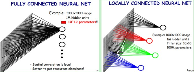
　　One such system is multilayer perceptrons aka neural networks which are multiple layers of neurons densely connected to each other. A deep vanilla neural network has such a large number of parameters involved that it is impossible to train such a system without overfitting the model due to the lack of a sufficient number of training examples. But with Convolutional Neural Networks(ConvNets), the task of training the whole network from the scratch can be carried out using a large dataset like ImageNet. The reason behind this is, sharing of parameters between the neurons and sparse connections in convolutional layers. It can be seen in this figure 2. In the convolution operation, the neurons in one layer are only locally connected to the input neurons and the set of parameters are shared across the 2-D feature map.

　　In order to understand the design philosophy of ConvNets, one must ask: What is the objective here ?  

　　a. Accuracy :

　　If you are building an intelligent machine, it is absolutely critical that it must be as accurate as possible. One fair question to ask here is that ‘accuracy not only depends on the network but also on the amount of data available for training’. Hence, these networks are compared on a standard dataset called ImageNet.

　　ImageNet project is an ongoing effort and currently has 14,197,122 images from 21841 different categories. Since 2010, ImageNet has been running an annual competition in visual recognition where participants are provided with 1.2 million images belonging to 1000 different classes from Imagenet data-set. So, each network architecture reports accuracy using these 1.2 million images of 1000 classes.

　　b. Computation:

　　Most ConvNets have huge memory and computation requirements, especially while training. Hence, this becomes an important concern. Similarly, the size of the final trained model becomes an important to consider if you are looking to deploy a model to run locally on mobile. As you can guess, it takes a more computationally intensive network to produce more accuracy. So, there is always a trade-off between accuracy and computation.

　　Apart from these, there are many other factors like ease of training, the ability of a network to generalize well etc. The networks described below are the most popular ones and are presented in the order that they were published and also had increasingly better accuracy from the earlier ones.

AlexNet

This architecture was one of the first deep networks to push ImageNet Classification accuracy by a significant stride in comparison to traditional methodologies. It is composed of 5 convolutional layers followed by 3 fully connected layers, as depicted in Figure 1.

 

 

 

AlexNet, proposed by Alex Krizhevsky, uses ReLu(Rectified Linear Unit) for the non-linear part, instead of a Tanh or Sigmoid function which was the earlier standard for traditional neural networks. ReLu is given by

f(x) = max(0,x)

The advantage of the ReLu over sigmoid is that it trains much faster than the latter because the derivative of sigmoid becomes very small in the saturating region and therefore the updates to the weights almost vanish(Figure 4). This is called vanishing gradient problem.

In the network, ReLu layer is put after each and every convolutional and fully-connected layers(FC).

Another problem that this architecture solved was reducing the over-fitting by using a Dropout layer after every FC layer. Dropout layer has a probability,(p), associated with it and is applied at every neuron of the response map separately. It randomly switches off the activation with the probability p, as can be seen in figure 5.

 

Why does DropOut work?

The idea behind the dropout is similar to the model ensembles. Due to the dropout layer, different sets of neurons which are switched off, represent a different architecture and all these different architectures are trained in parallel with weight given to each subset and the summation of weights being one. For n neurons attached to DropOut, the number of subset architectures formed is 2^n. So it amounts to prediction being averaged over these ensembles of models. This provides a structured model regularization which helps in avoiding the over-fitting. Another view of DropOut being helpful is that since neurons are randomly chosen, they tend to avoid developing co-adaptations among themselves thereby enabling them to develop meaningful features, independent of others.

VGG16

This architecture is from VGG group, Oxford. It makes the improvement over AlexNet by replacing large kernel-sized filters(11 and 5 in the first and second convolutional layer, respectively) with multiple 3X3 kernel-sized filters one after another. With a given receptive field(the effective area size of input image on which output depends), multiple stacked smaller size kernel is better than the one with a larger size kernel because multiple non-linear layers increases the depth of the network which enables it to learn more complex features, and that too at a lower cost.

For example, three 3X3 filters on top of each other with stride 1 ha a receptive size of 7, but the number of parameters involved is 3*(9C^2) in comparison to 49C^2 parameters of kernels with a size of 7. Here, it is assumed that the number of input and output channel of layers is C.Also, 3X3 kernels help in retaining finer level properties of the image. The network architecture is given in the table.

　　

You can see that in VGG-D, there are blocks with same filter size applied multiple times to extract more complex and representative features. This concept of blocks/modules became a common theme in the networks after VGG.

The VGG convolutional layers are followed by 3 fully connected layers. The width of the network starts at a small value of 64 and increases by a factor of 2 after every sub-sampling/pooling layer. It achieves the top-5 accuracy of 92.3 % on ImageNet.

GoogLeNet/Inception:

While VGG achieves a phenomenal accuracy on ImageNet dataset, its deployment on even the most modest sized GPUs is a problem because of huge computational requirements, both in terms of memory and time. It becomes inefficient due to large width of convolutional layers.

For instance, a convolutional layer with 3X3 kernel size which takes 512 channels as input and outputs 512 channels, the order of calculations is 9X512X512.

In a convolutional operation at one location, every output channel (512 in the example above), is connected to every input channel, and so we call it a dense connection architecture. The GoogLeNet builds on the idea that most of the activations in deep network are either unnecessary(value of zero) or redundant because of correlations between them. Therefore most efficient architecture of a deep network will have a sparse connection between the activations, which implies that all 512 output channels will not have a connection with all the 512 input channels. There are techniques to prune out such connections which would result in a sparse weight/connection. But kernels for sparse matrix multiplication are not optimized in BLAS or CuBlas(CUDA for GPU) packages which render them to be even slower than their dense counterparts.

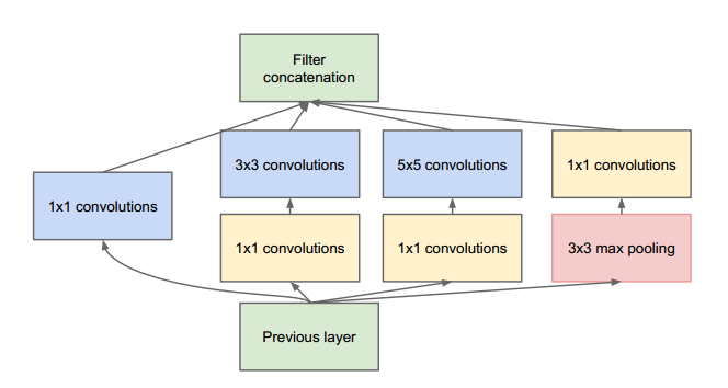
So GoogLeNet devised a module called inception module that approximates a sparse CNN with a normal dense construction(shown in the figure). Since only a small number of neurons are effective as mentioned earlier, width/number of the convolutional filters of a particular kernel size is kept small. Also, it uses convolutions of different sizes to capture details at varied scales(5X5, 3X3, 1X1).

Another salient point about the module is that it has a so-called bottleneck layer (1X1 convolutions in the figure). It helps in massive reduction of the computation requirement as explained below.

Let us take the first inception module of GoogLeNet as an example which has 192 channels as input. It has just 128 filters of 3X3 kernel size and 32 filters of 5X5 size. The order of computation for 5X5 filters is 25X32X192 which can blow up as we go deeper into the network when the width of the network and the number of 5X5 filter further increases. In order to avoid this, the inception module uses 1X1 convolutions before applying larger sized kernels to reduce the dimension of the input channels, before feeding into those convolutions. So in first inception module, the input to the module is first fed into 1X1 convolutions with just 16 filters before it is fed into 5X5 convolutions. This reduces the computations to 16X192 +  25X32X16. All these changes allow the network to have a large width and depth.

Another change that GoogLeNet made, was to replace the fully-connected layers at the end with a simple global average pooling which averages out the channel values across the 2D feature map, after the last convolutional layer. This drastically reduces the total number of parameters. This can be understood from AlexNet, where FC layers contain approx. 90% of parameters. Use of a large network width and depth allows GoogLeNet to remove the FC layers without affecting the accuracy. It achieves 93.3% top-5 accuracy on ImageNet and is much faster than VGG.

Residual Networks

As per what we have seen so far, increasing the depth should increase the accuracy of the network, as long as over-fitting is taken care of. But the problem with increased depth is that the signal required to change the weights, which arises from the end of the network by comparing ground-truth and prediction becomes very small at the earlier layers, because of increased depth. It essentially means that earlier layers are almost negligible learned. This is called vanishing gradient. The second problem with training the deeper networks is, performing the optimization on huge parameter space and therefore naively adding the layers leading to higher training error. Residual networks allow training of such deep networks by constructing the network through modules called residual models as shown in the figure. This is called degradation problem. The intuition around why it works can be seen as follows:

 

 

Imagine a network, A which produces x amount of training error. Construct a network B by adding few layers on top of A and put parameter values in those layers in such a way that they do nothing to the outputs from A. Let’s call the additional layer as C. This would mean the same x amount of training error for the new network. So while training network B, the training error should not be above the training error of A. And since it DOES happen, the only reason is that learning the identity mapping(doing nothing to inputs and just copying as it is) with the added layers-C is not a trivial problem, which the solver does not achieve. To solve this, the module shown above creates a direct path between the input and output to the module implying an identity mapping and the added layer-C just need to learn the features on top of already available input. Since C is learning only the residual, the whole module is called residual module.

Also, similar to GoogLeNet, it uses a global average pooling followed by the classification layer.Through the changes mentioned, ResNets were learned with network depth of as large as 152. It achieves better accuracy than VGGNet and GoogLeNet while being computationally more efficient than VGGNet. ResNet-152 achieves 95.51 top-5 accuracies.

The architecture is similar to the VGGNet consisting mostly of 3X3 filters. From the VGGNet, shortcut connection as described above is inserted to form a residual network. This can be seen in the figure which shows a small snippet of earlier layer synthesis from VGG-19.

The power of the residual networks can be judged from one of the experiments in paper 4. The plain 34 layer network had higher validation error than the 18 layer plain network. This is where we realize the degradation problem. And the same 34 layer network when converted into the residual network has much lesser training error than the 18 layer residual network. 

 

 

As we design more and more sophisticated architectures, some of the networks may not stay relevant few years down the line but the core priciples that led to their design must be understood. Hope this articles offered you a good perspective into the design of neural network architectures.