『科学计算』通过代码理解SoftMax多分类

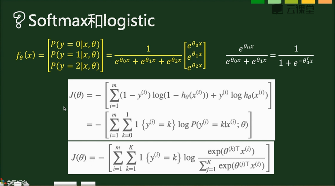
SoftMax实际上是Logistic的推广，当分类数为2的时候会退化为Logistic分类

其计算公式和损失函数如下，

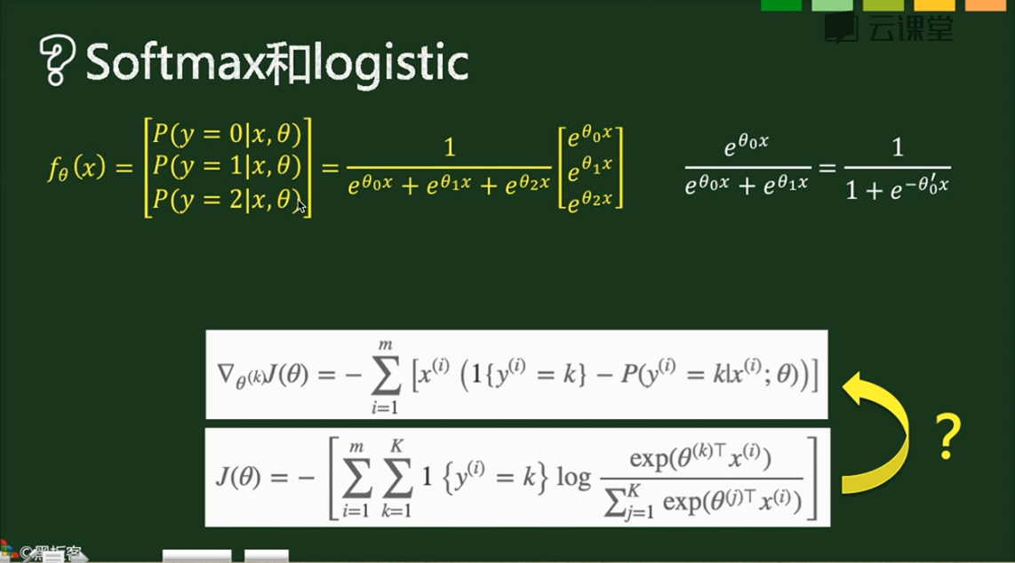
梯度如下，

1{条件} 表示True为1，False为0，在下图中亦即对于每个样本只有正确的分类才取1，对于损失函数实际上只有m个表达式（m个样本每个有一个正确的分类）相加，

对于梯度实际上是把我们以前的最后一层和分类层合并了：

• 第一步则和之前的求法类似，1-概率 & 0-概率组成向量，作为分类层的梯度，对batch数据实现的话就是建立一个(m,k)的01矩阵，直接点乘控制开关，最后求np.sum
• x的转置乘分类层梯度
• 全batch数据求和，实际上这在代码实现中和上一步放在了一块

对于单个数据梯度：x.T.dot(y_pred-y)，维度是这样的(k,1)*(1,c)=(k,c)

对于成批数据梯度：X.T.dot(y_pred-y)，维度是这样的(k,m)*(1,c)=(k,c)，只不过结果矩阵的对应位置由x(i,1)*er(1,j)变换为x0(i,1)*er(1,j)+x1(i,1)*er(1,j)... ...正好是对全batch求了个和，所以后面需要除下去

X.T.dot(grad_next)结果是batch梯度累加和，所以需要除以样本数m，这个结论对全部使用本公式的梯度均成立（1，这句话是废话；2，但是几乎全部机器or深度学习算法都需要矩阵乘法，亦即梯度必须使用本公式，所以是很重要的废话）。

L2正则化：lamda*np.sum(W*W)或者lamda*np.sum(W.T.dot(W))均可，实际上就是W各个项的平方和

#计算Error，Cost，Grad
y_dash = self.softmax(X.dot(theta_n))   # 向前传播结果

Y = np.zeros((m,10))                    # one-hot编码label矩阵
for i in range(m):
    Y[i,y[i]]=1

error = np.sum(Y * np.log(y_dash), axis=1)   # 注意，这里是点乘
cost = -np.sum(error, axis=0)
grad = X.T.dot(y_dash-Y)

grad_n = grad.ravel()

代码实现：

import numpy as np
import matplotlib.pyplot as plt
import math

def scale_n(x):
    return x
    #return (x-x.mean(axis=0))/(x.std(axis=0)+1e-10)

class SoftMaxModel(object):
    def __init__(self,alpha=0.06,threhold=0.0005):
        self.alpha = alpha         # 学习率
        self.threhold = threhold   # 循环终止阈值
        self.num_classes = 10      # 分类数

    def setup(self,X):
        # 初始化权重矩阵，注意，由于是多分类，所以权重由向量变化为矩阵
        # 而且这里面初始化的是flat为1维的矩阵
        m, n = X.shape  # 400,15
        s = math.sqrt(6) / math.sqrt(n+self.num_classes)
        theta = np.random.rand(n*(self.num_classes))*2*s-s  #[15,1]
        return theta

    def softmax(self,x):
        # 先前传播softmax多分类
        # 注意输入的x是[batch数目n，类数目m]，输出是[batch数目n，类数目m]
        e = np.exp(x)
        temp = np.sum(e, axis=1,keepdims=True)
        return e/temp

    def get_cost_grad(self,theta,X,y):
        m, n = X.shape
        theta_n = theta.reshape(n, self.num_classes)

        #计算Error，Cost，Grad
        y_dash = self.softmax(X.dot(theta_n))   # 向前传播结果

        Y = np.zeros((m,10))                    # one-hot编码label矩阵
        for i in range(m):
            Y[i,y[i]]=1

        error = np.sum(Y * np.log(y_dash), axis=1)
        cost = -np.sum(error, axis=0)
        grad = X.T.dot(y_dash-Y)

        grad_n = grad.ravel()
        return cost,grad_n

    def train(self,X,y,max_iter=50, batch_size=200):
        m, n = X.shape  # 400,15
        theta = self.setup(X)

        #our intial prediction
        prev_cost = None
        loop_num = 0
        n_samples = y.shape[0]
        n_batches = n_samples // batch_size
        # Stochastic gradient descent with mini-batches
        while loop_num < max_iter:
            for b in range(n_batches):
                batch_begin = b*batch_size
                batch_end = batch_begin+batch_size
                X_batch = X[batch_begin:batch_end]
                Y_batch = y[batch_begin:batch_end]

                #intial cost
                cost,grad = self.get_cost_grad(theta,X_batch,Y_batch)

                theta = theta- self.alpha * grad/float(batch_size)

            loop_num+=1
            if loop_num%10==0:
                print (cost,loop_num)
            if prev_cost:
                if prev_cost - cost <= self.threhold:
                    break

            prev_cost = cost

        self.theta = theta
        print (theta,loop_num)

    def train_scipy(self,X,y):
        m,n = X.shape
        import scipy.optimize
        options = {'maxiter': 50, 'disp': True}
        J = lambda x: self.get_cost_grad(x, X, y)
        theta = self.setup(X)

        result = scipy.optimize.minimize(J, theta, method='L-BFGS-B', jac=True, options=options)
        self.theta = result.x

    def predict(self,X):
        m,n = X.shape
        theta_n = self.theta.reshape(n, self.num_classes)
        a = np.argmax(self.softmax(X.dot(theta_n)),axis=1)
        return a

    def grad_check(self,X,y):
        epsilon = 10**-4
        m, n = X.shape   

        sum_error=0
        N=300

        for i in range(N):
            theta = self.setup(X)
            j = np.random.randint(1,len(theta))
            theta1=theta.copy()
            theta2=theta.copy()
            theta1[j]+=epsilon
            theta2[j]-=epsilon

            cost1,grad1 = self.get_cost_grad(theta1,X,y)
            cost2,grad2 = self.get_cost_grad(theta2,X,y)
            cost3,grad3 = self.get_cost_grad(theta,X,y)

            sum_error += np.abs(grad3[j]-(cost1-cost2)/float(2*epsilon))
        print ("grad check error is %e\n"%(sum_error/float(N)))

if __name__=="__main__":

    import cPickle, gzip
    # Load the dataset
    f = gzip.open('mnist.pkl.gz', 'rb')
    train_set, valid_set, test_set = cPickle.load(f)
    f.close()
    train_X = scale_n(train_set[0])
    train_y = train_set[1]
    test_X = scale_n(test_set[0])
    test_y = test_set[1]

    l_model = SoftMaxModel()

    l_model.grad_check(test_X[0:200,:],test_y[0:200])

    l_model.train_scipy(train_X,train_y)

    predict_train_y = l_model.predict(train_X)
    b = predict_train_y!=train_y

    error_train = np.sum(b, axis=0)/float(b.size)    

    predict_test_y = l_model.predict(test_X)
    b = predict_test_y!=test_y

    error_test = np.sum(b, axis=0)/float(b.size)

    print ("Train Error rate = %.4f, \nTest Error rate = %.4f\n"%(error_train,error_test))

这里面有scipy的优化器应用，因为不是重点（暂时没有学习这个库的日程），所以标注出来，需要用优化器优化函数的时候记得有这么回事再深入学习即可：

def train_scipy(self,X,y):
        m,n = X.shape
        import scipy.optimize
        options = {'maxiter': 50, 'disp': True}
        J = lambda x: self.get_cost_grad(x, X, y)
        theta = self.setup(X)

        result = scipy.optimize.minimize(J, theta, method='L-BFGS-B', jac=True, options=options)
        self.theta = result.x

主要是提供了一些比较复杂的优化算法，而且是一个优化自建目标函数的demo，以后可能有所应用。