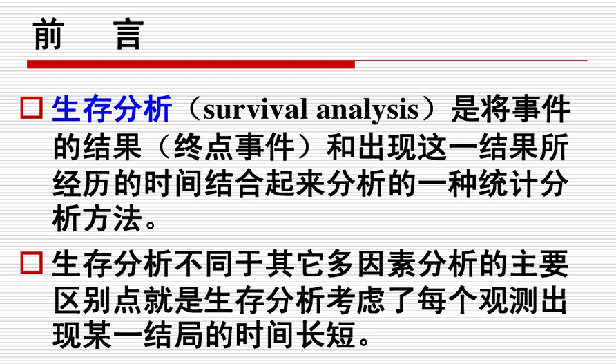
生存分析/Weibull Distribution韦布尔分布

 python机器学习-乳腺癌细胞挖掘（博主亲自录制视频）

https://study.163.com/course/introduction.htm?courseId=1005269003&utm_campaign=commission&utm_source=cp-400000000398149&utm_medium=share

机器学习，统计项目合作请联系

QQ：231469242

测试脚本

测试数据

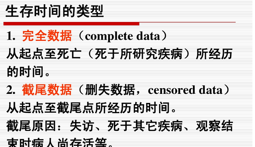
T is an array of durations, E is a either boolean or binary array representing whether the “death” was observed (alternatively an individual can be censored).

import lifelines
from lifelines.datasets import load_waltons
 
df = load_waltons() # returns a Pandas DataFrame
 
T = df['T']
E = df['E']
 
from lifelines import KaplanMeierFitter
kmf = KaplanMeierFitter()
kmf.fit(T, event_observed=E) # more succiently, kmf.fit(T,E)
 
kmf.survival_function_
'''
Out[7]:
          KM_estimate
timeline
0.0          1.000000
6.0          0.993865
7.0          0.987730
9.0          0.969210
13.0         0.950690
15.0         0.938344
17.0         0.932170
19.0         0.913650
22.0         0.888957
26.0         0.858090
29.0         0.827224
32.0         0.821051
33.0         0.802531
36.0         0.790184
38.0         0.777837
41.0         0.734624
43.0         0.728451
45.0         0.672891
47.0         0.666661
48.0         0.616817
51.0         0.598125
 
'''
 
kmf.median_
'''
Out[8]: 56.0
'''
kmf.plot()

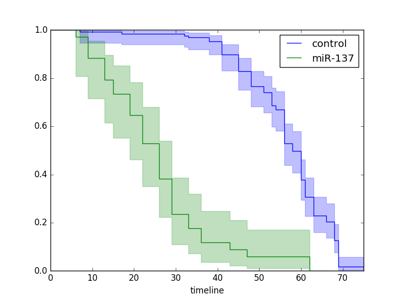
import lifelines
from lifelines.datasets import load_waltons
from lifelines import KaplanMeierFitter
df = load_waltons() # returns a Pandas DataFrame
 
kmf = KaplanMeierFitter()
T = df['T']
E = df['E']
groups = df['group']
ix = (groups == 'miR-137')
 
kmf.fit(T[~ix], E[~ix], label='control')
ax = kmf.plot()
 
kmf.fit(T[ix], E[ix], label='miR-137')
kmf.plot(ax=ax)

import numpy as np
import matplotlib.pyplot as plt
from lifelines.plotting import plot_lifetimes
from numpy.random import uniform, exponential
 
N = 25
current_time = 10
actual_lifetimes = np.array([[exponential(12), exponential(2)][uniform()<0.5] for i in range(N)])
observed_lifetimes = np.minimum(actual_lifetimes,current_time)
observed= actual_lifetimes < current_time
 
plt.xlim(0,25)
plt.vlines(10,0,30,lw=2, linestyles="--")
plt.xlabel('time')
plt.title('Births and deaths of our population, at $t=10$')
plot_lifetimes(observed_lifetimes, event_observed=observed)
print "Observed lifetimes at time %d:\n"%(current_time), observed_lifetimes

import pandas as pd
import lifelines
from lifelines import KaplanMeierFitter
import matplotlib.pyplot as plt
 
data = lifelines.datasets.load_dd()
kmf = KaplanMeierFitter()
 
T = data["duration"]
C = data["observed"]
 
kmf.fit(T, event_observed=C )
plt.title('Survival function of political regimes')
kmf.survival_function_.plot()
kmf.plot()
 
kmf.median_

import pandas as pd
import lifelines
from lifelines import KaplanMeierFitter
import matplotlib.pyplot as plt
 
data = lifelines.datasets.load_dd()
kmf = KaplanMeierFitter()
 
T = data["duration"]
C = data["observed"]
 
kmf.fit(T, event_observed=C )
plt.title('Survival function of political regimes')
kmf.survival_function_.plot()
kmf.plot()
 
ax = plt.subplot(111)
 
dem = (data["democracy"] == "Democracy")
kmf.fit(T[dem], event_observed=C[dem], label="Democratic Regimes")
kmf.plot(ax=ax, ci_force_lines=True)
kmf.fit(T[~dem], event_observed=C[~dem], label="Non-democratic Regimes")
 
plt.ylim(0,1);
plt.title("Lifespans of different global regimes")
kmf.plot(ax=ax, ci_force_lines=True)

应用于保险业，病人治疗，信用卡诈骗

信用卡拖欠

具体文档

http://lifelines.readthedocs.io/en/latest/

https://wenku.baidu.com/view/577041d3a1c7aa00b52acb2e.html?from=search

https://wenku.baidu.com/view/a5adff8b89eb172ded63b7d6.html?from=search

https://github.com/thomas-haslwanter/statsintro_python/tree/master/ISP/Code_Quantlets/10_SurvivalAnalysis/lifelinesDemo

测试代码

# -*- coding: utf-8 -*-
# Import standard packages
import numpy as np
import matplotlib.pyplot as plt
from numpy.random import uniform, exponential
import os
 
# additional packages
from lifelines.plotting import plot_lifetimes
import sys
sys.path.append(os.path.join('..', '..', 'Utilities'))
 
try:
# Import formatting commands if directory "Utilities" is available
    from ISP_mystyle import setFonts
 
except ImportError:
# Ensure correct performance otherwise
    def setFonts(*options):
        return
 
# Generate some dummy data
np.set_printoptions(precision=2)
N = 20
study_duration = 12
 
# Note: a constant dropout rate is equivalent to an exponential distribution!
actual_subscriptiontimes = np.array([[exponential(18), exponential(3)][uniform()<0.5] for i in range(N)])
observed_subscriptiontimes = np.minimum(actual_subscriptiontimes,study_duration)
observed= actual_subscriptiontimes < study_duration
 
# Show the data
setFonts(18)
plt.xlim(0,24)
plt.vlines(12, 0, 30, lw=2, linestyles="--")
plt.xlabel('time')
plt.title('Subscription Times, at $t=12$  months')
plot_lifetimes(observed_subscriptiontimes, event_observed=observed)
 
print("Observed subscription time at time %d:\n"%(study_duration), observed_subscriptiontimes)

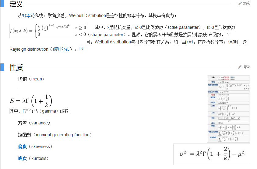
where k > 0 is the shape parameter and > 0 is the scale parameter of the
distribution. (It is one of the rare cases where we use a shape parameter different
from skewness and kurtosis.) Its complementary cumulative distribution function is
a stretched exponential function.
If the quantity x is a “time-to-failure,” theWeibull distribution gives a distribution
for which the failure rate is proportional to a power of time. The shape parameter, k,
is that power plus one, and so this parameter can be interpreted directly as follows:
• Avalueofk < 1 indicates that the failure rate decreases over time. This happens
if there is significant “infant mortality,” or defective items failing early and the
failure rate decreasing over time as the defective items are weeded out of the
population.
• Avalueofk D 1 indicates that the failure rate is constant over time. This might
suggest random external events are causing mortality, or failure.
• Avalueofk > 1 indicates that the failure rate increases with time. This happens
if there is an “aging” process, or parts that are more likely to fail as time goes on.
An example would be products with a built-in weakness that fail soon after the
warranty expires.
In the field of materials science, the shape parameter k of a distribution of
strengths is known as the Weibull modulus.

威布尔分布（Weibull distribution），又称韦伯分布或韦布尔分布，是可靠性分析和寿命检验的理论基础。

威布尔分布：在可靠性工程中被广泛应用，尤其适用于机电类产品的磨损累计失效的分布形式。由于它可以利用概率值很容易地推断出它的分布参数，被广泛应用于各种寿命试验的数据处理。

 

随机变量分布之一。威布尔分布(Ⅲ型 极值分布)记为W(k,a,b)。
　
　瑞典工程师威布尔从30年代开始研究轴承寿命，以后又研究结构强度和疲劳等问题。他采用了“链式”模型来解释结构强度和寿命问题。这个模型假设一个结构
是由若干小元件(设为n个)串联而成，于是可以形象地将结构看成是由n个环构成的一条链条，其强度(或寿命)取决于最薄弱环的强度(或寿命)。单个链的强
度(或寿命)为一随机变量，设各环强度(或寿命)相互独立，分布相同，则求链强度(或寿命)的概率分布就变成求极小值分布问题，由此给出威布尔分布函数。
由于零件或结构的疲劳强度(或寿命)也应取决于其最弱环的强度(或寿命)，也应能用威布尔分布描述。
　　根据1943年苏联格涅坚科的研究结果，不管随机变量的原始分布如何，它的极小值的渐近分布只能有三种，而威布尔分布就是第Ⅲ种极小值分布。
　　由于威布尔分布是根据最弱环节模型或串联模型得到的，能充分反映材料缺陷和应力集中源对材料疲劳寿命的影响，而且具有递增的失效率，所以，将它作为材料或零件的寿命分布模型或给定寿命下的疲劳强度模型是合适的。
　
　威布尔分布有多种形式，包括一参数威布尔分布、二参数威布尔分布、三参数威布尔分布或混合威布尔分布。三参数的威布尔分布由形状、尺度（范围）和位置三
个参数决定。其中形状参数是最重要的参数，决定分布密度曲线的基本形状，尺度参数起放大或缩小曲线的作用，但不影响分布的形状。通过改变形状参数可以表示
不同阶段的失效情况；也可以作为许多其他分布的近似，如，可将形状参数设为合适的值以近似正态、对数正态、指数等分布。

二参数的威布尔分布主要用于滚动轴承的寿命试验以及高应力水平下的材料疲
劳试验，三参数的威布尔分布用于低应力水平的材料及某些零件的寿命试验，一般而言，它具有比对数正态分布更大的适用性。但是，威布尔分布参数的分析法估计
较复杂，区间估计值过长，实践中常采用概率纸估计法，从而降低了参数的估计精度．这是威布尔分布目前存在的主要缺点，也限制了它的应用^[1] 

 

历史

编辑

1. 1927年，Fréchet(1927)首先给出这一分布的定义。

2. 1933年，Rosin和Rammler在研究碎末的分布时，第一次应用了韦伯分布（Rosin, P.; Rammler, E. (1933), "The Laws Governing the Fineness of Powdered Coal", Journal of the Institute of Fuel 7: 29 - 36.）。

3. 1951年，瑞典工程师、数学家Waloddi Weibull（1887-1979）详细解释了这一分布，于是，该分布便以他的名字命名为Weibull Distribution。

应用

编辑

1.生存分析

2.工业制造

研究生产过程和运输时间关系

3.极值理论

4.预测天气

5.可靠性和失效分析

6.雷达系统

对接受到的杂波信号的依分布建模

7.拟合度

无线通信技术中，相对指数衰减频道模型，Weibull衰减模型对衰减频道建模有较好的拟合度

8.量化寿险模型的重复索赔

9.预测技术变革

10.风速

由于曲线形状与现实状况很匹配，被用来描述风速的分布

 

 

 

4

 

 

 

 

 

 

 

 

 

 

 

 

 

 

 

 

 

 

 

 

 

 

 

 

 

 

 

 

 

 

 

 

 

 

 

 

 

 

 

 

 

 

 

 

 

https://study.163.com/provider/400000000398149/index.htm?share=2&shareId=400000000398149（ 欢迎关注博主主页，学习python视频资源，还有大量免费python经典文章）