『MXNet』第十弹_物体检测SSD

全流程地址

一、辅助API介绍

mxnet.image.ImageDetIter

图像检测迭代器，

from mxnet import image
from mxnet import nd

data_shape = 256
batch_size = 32
rgb_mean = nd.array([123, 117, 104])

def get_iterators(data_shape, batch_size):
    """256, 32"""
    class_names = ['pikachu']
    num_class = len(class_names)
    train_iter = image.ImageDetIter(
        batch_size=batch_size,
        data_shape=(3, data_shape, data_shape),
        path_imgrec=data_dir+'train.rec',
        path_imgidx=data_dir+'train.idx',
        shuffle=True,
        mean=True,
        rand_crop=1,
        min_object_covered=0.95,
        max_attempts=200)
    val_iter = image.ImageDetIter(
        batch_size=batch_size,
        data_shape=(3, data_shape, data_shape),
        path_imgrec=data_dir+'val.rec',
        shuffle=False,
        mean=True)
    return train_iter, val_iter, class_names, num_class

train_data, test_data, class_names, num_class = get_iterators(
    data_shape, batch_size)

batch = train_data.next()
# (32, 1, 5)
# 1：图像中只有一个目标
# 5：第一个元素对应物体的标号，-1表示非法物体；后面4个元素表示边框，0~1
# 多个目标时list[nd(batch_size, 目标数目, 目标信息)]
print(batch)
# list[nd(batch_size,channel,width,higth)]
print(batch.data[0].shape)
print(batch.label[0].shape)

DataBatch: data shapes: [(32, 3, 256, 256)] label shapes: [(32, 1, 5)]
(32, 3, 256, 256)
(32, 1, 5)

可以看到标号的形状是batch_size x num_object_per_image x 5。这里数据里每个图片里面只有一个标号。每个标号由长为5的数组表示，第一个元素是其对用物体的标号，其中-1表示非法物体，仅做填充使用。后面4个元素表示边框。

mxnet.metric

from mxnet import metric

cls_metric = metric.Accuracy()
box_metric = metric.MAE() 

cls_metric.update([cls_target], [class_preds.transpose((0,2,1))])
box_metric.update([box_target], [box_preds * box_mask])
cls_metric.get()
box_metric.get()

gluon.loss.Loss

用法类似Block，被继承用来定义新的损失函数，值得注意的是这里体现了F的用法：代替mx.nd or mx.sym

class FocalLoss(gluon.loss.Loss):
    def __init__(self, axis=-1, alpha=0.25, gamma=2, batch_axis=0, **kwargs):
        super(FocalLoss, self).__init__(None, batch_axis, **kwargs)
        self._axis = axis
        self._alpha = alpha
        self._gamma = gamma

    def hybrid_forward(self, F, output, label):
        # (32, 5444, 2) (32, 5444)
        # Here `F` can be either mx.nd or mx.sym
        # 这里使用F取代在forward中显式的指定两者，方便使用
        # 所以非hybrid无此参数
        output = F.softmax(output)
        pj = output.pick(label, axis=self._axis, keepdims=True)
        # print(pj.shape)  (32, 5444, 1)：仅仅保留正确类别对应的概率
        # print(self._axis)  -1
        loss = - self._alpha * ((1 - pj) ** self._gamma) * pj.log()
        return loss.mean(axis=self._batch_axis, exclude=True)

pick：根据label最后一维的值选取output的-2维上的元素

二、框体处理系列函数

框体生成：mxnet.contrib.ndarray.MultiBoxPrior

因为边框可以出现在图片中的任何位置，并且可以有任意大小。为了简化计算，SSD跟Faster R-CNN一样使用一些默认的边界框，或者称之为锚框（anchor box），做为搜索起点。具体来说，对输入的每个像素，以其为中心采样数个有不同形状和不同比例的边界框。假设输入大小是 w×hw×h，

• 给定大小 s∈(0,1]s∈(0,1]，那么生成的边界框形状是 
• 给定比例 r>0r>0，那么生成的边界框形状是 

在采样的时候我们提供 n 个大小（sizes）和 m 个比例（ratios）。为了计算简单这里不生成nm个锚框，而是n+m−1个。其中第 i 个锚框使用

• sizes[i]和ratios[0] 如果 i≤n
• sizes[0]和ratios[i-n] 如果 i>n

我们可以使用contribe.ndarray里的MultiBoxPrior来采样锚框。这里锚框通过左下角和右上角两个点来确定，而且被标准化成了区间[0,1][0,1]的实数。

from mxnet import nd
from mxnet.contrib.ndarray import MultiBoxPrior

# shape: batch x channel x height x weight
n = 40
x = nd.random.uniform(shape=(1, 3, n, n))

y = MultiBoxPrior(x, sizes=[.5,.25,.1], ratios=[1,2,.5])
# 每个像素点(n*n)，5个框，4个坐标值
boxes = y.reshape((n, n, -1, 4))
print(boxes.shape)
# The first anchor box centered on (20, 20)
# its format is (x_min, y_min, x_max, y_max)
boxes[20, 20, :, :]

(40, 40, 5, 4)

Out[5]:

[[ 0.26249999  0.26249999  0.76249999  0.76249999]
 [ 0.38749999  0.38749999  0.63749999  0.63749999]
 [ 0.46249998  0.46249998  0.5625      0.5625    ]
 [ 0.1589466   0.33572328  0.86605334  0.6892767 ]
 [ 0.33572328  0.1589466   0.6892767   0.86605334]]
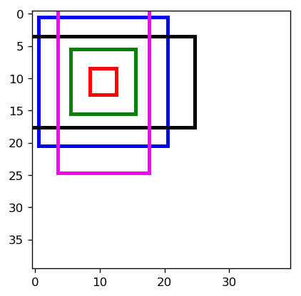
<NDArray 5x4 @cpu(0)>我们可以画出以(20,20)为中心的所有锚框：

colors = ['blue', 'green', 'red', 'black', 'magenta']

# 白板背景
plt.imshow(nd.ones((n, n, 3)).asnumpy())
# 提取某个像素点的框子
anchors = boxes[10, 10, :, :]
for i in range(anchors.shape[0]):
    plt.gca().add_patch(box_to_rect(anchors[i,:]*n, colors[i]))
plt.show()
# 可以看到，贴边框子会被截断

框体筛选：mxnet.contrib.ndarray.MultiBoxTarget

虽然每张图片里面通常只有几个标注的边框，但SSD会生成大量的锚框。可以想象很多锚框都不会框住感兴趣的物体，就是说跟任何对应感兴趣物体的表框的IoU都小于某个阈值。这样就会产生大量的负类锚框，或者说对应标号为0的锚框。对于这类锚框有两点要考虑的：

1. 边框预测的损失函数不应该包括负类锚框，因为它们并没有对应的真实边框
2. 因为负类锚框数目可能远多于其他，我们可以只保留其中的一些。而且是保留那些目前预测最不确信它是负类的，就是对类0预测值排序，选取数值最小的哪一些困难的负类锚框。

我们可以使用MultiBoxTarget来完成上面这两个操作。

def training_targets(anchors, class_preds, labels):
    """
    得到的全部边框坐标
    得到的全部边框各个类别得分
    真实类别及对应边框坐标
    """
    class_preds = class_preds.transpose(axes=(0,2,1))
    return MultiBoxTarget(anchors, labels, class_preds)

# Output achors: (1, 5444, 4)，1张图共5444个框4个坐标值
# Output class predictions: (1, 5444, 3)，1张图5444个框3个类别(2分类+背景)
# batch.label: (1, 1, 5)，1张图1个对象(1具体类别+4坐标)
out = training_targets(anchors, class_preds, batch.label[0][0:1])

[[ 0.  0.  0. ...,  0.  0.  0.]]

它返回三个NDArray，分别是

1. 预测的边框跟真实边框的偏移，大小是batch_size x (num_anchors*4)
2. 用来遮掩不需要的负类锚框的掩码，大小跟上面一致
3. 锚框的真实的标号，大小是batch_size x num_anchors

我们可以计算这次只选中了多少个锚框进入损失函数：

out[1].sum()/4

[ 14.]
<NDArray 1 @cpu(0)>

这里不太直观，我们看看网络中调用：

box_target, box_mask, cls_target = training_targets(
                anchors, class_preds, y)
# IN：
# anchors(1, 5444, 4): 1, 框子数， 坐标数
# 各个框体原本坐标
# class_preds(32, 5444, 2)：batch，框子数，类别数  cls_loss
# 各个框体分类信息
# y(32, 3, 5)：batch，对象数，对象信息(类别+坐标)
# 真实标签
# OUT：
# box_target(32, 21776)：batch，框子数*坐标数  box_loss
# 每个坐标框相较于真实框的偏移，作为被学习标签
# box_mask(32, 21776) ：batch，框子数*坐标数  box_loss
# 每一个框每一个坐标是否保留(是1否0)
# cls_target(32, 5444)：batch，框子数  cls_loss
# 每一个框对应的真实类别序号(背景0)

实际上anchors(即mxnet.contrib.ndarray.MultiBoxTarget于各个回归层生成)是固定不变的，我们使用每一个框子anchors、该框对应的的预测值class_preds、真实框标签得到：

• 每一个框体坐标偏移，经过了阈值检查的，默认overlap_threshold=0.5(值约小阈值越高)
• 这些框体的掩码(就是上面向量非零值替换为1，预测基本不会没有偏差)
• 每一个框子对应的类别，和上面非0输出数目保持一致

非极大值抑制：mxnet.contrib.ndarray.MultiBoxDetection

因为我们对每个像素都会生成数个锚框，这样我们可能会预测出大量相似的表框，从而导致结果非常嘈杂。一个办法是对于IoU比较高的两个表框，我们只保留预测执行度比较高的那个。这个算法（称之为non maximum suppression）在MultiBoxDetection里实现，

from mxnet.contrib.ndarray import MultiBoxDetection

def predict(x):
    anchors, cls_preds, box_preds = net(x.as_in_context(ctx))
    # anchors.shape, class_preds.shape, box_preds.shape
    # (1, 5444, 4)   (32, 5444, 2)      (32, 21776) box_loss
    cls_probs = nd.SoftmaxActivation(
        cls_preds.transpose((0,2,1)), mode='channel')

    return MultiBoxDetection(cls_probs, box_preds, anchors,
                             force_suppress=True, clip=False)

可以看到，函数接收各个框体分类信息，各个框体回归(修正)信息，各个框体原本坐标，

对应的它输出所有边框，每个边框由[class_id, confidence, xmin, ymin, xmax, ymax]表示。其中class_id=-1表示要么这个边框被预测只含有背景，或者被去重掉了：

x, im = process_image('../img/pikachu.jpg')
out = predict(x)
out.shape

(1, 5444, 6)

三、网络主干

def class_predictor(num_anchors, num_classes):
    """return a layer to predict classes"""
    # 输入输出大小相同，输出的不同通道对应(不同框)的(不同类别)的得分
    # 输出图片每一个像素点上通道数：框体数目×(类别数 + 1，背景）
    return nn.Conv2D(num_anchors * (num_classes + 1), 3, padding=1)

def box_predictor(num_anchors):
    """return a layer to predict delta locations"""
    return nn.Conv2D(num_anchors * 4, 3, padding=1)

def down_sample(num_filters):
    """
    定义一个卷积块，它将输入特征的长宽减半，以此来获取多尺度的预测。它由两个Conv-BatchNorm-Relu
    组成，我们使用填充为1的3×33×3卷积使得输入和输入有同样的长宽，然后再通过跨度为2的最大池化层将长
    宽减半。
    """
    out = nn.HybridSequential()
    for _ in range(2):
        out.add(nn.Conv2D(num_filters, 3, strides=1, padding=1))
        out.add(nn.BatchNorm(in_channels=num_filters))
        out.add(nn.Activation('relu'))
    out.add(nn.MaxPool2D(2))
    return out

def flatten_prediction(pred):
    # 图片数，像素数×框数×分类数：值为得分
    return pred.transpose(axes=(0,2,3,1)).flatten()

def concat_predictions(preds):
    # 图片数，(全部层的)像素数×框数×分类数：值为得分
    return nd.concat(*preds, dim=1)

def body():
    """
    主体网络用来从原始像素抽取特征。通常前面介绍的用来图片分类的卷积神经网络，例如ResNet，
    都可以用来作为主体网络。这里为了示范，我们简单叠加几个减半模块作为主体网络。
    """
    out = nn.HybridSequential()
    for nfilters in [16, 32, 64]:
        out.add(down_sample(nfilters))
    return out

def toy_ssd_model(num_anchors, num_classes):
    """
    创建一个玩具SSD模型了。我们称之为玩具是因为这个网络不管是层数还是锚框个数都比较小，
    仅仅适合之后我们之后使用的一个小数据集。但这个模型不会影响我们介绍SSD。
    这个网络包含四块。主体网络，三个减半模块，以及五个物体类别和边框预测模块。其中预测分
    别应用在在主体网络输出，减半模块输出，和最后的全局池化层上。
    """
    # 含三个减半模块
    downsamplers = nn.Sequential()
    for _ in range(3):
        downsamplers.add(down_sample(128))
    # 含五个分类预测模块
    class_predictors = nn.Sequential()
    # 含五个边框回归模块
    box_predictors = nn.Sequential()
    for _ in range(5):
        class_predictors.add(class_predictor(num_anchors, num_classes))
        box_predictors.add(box_predictor(num_anchors))

    # 主体网络 + 减半 + 分类 + 回归
    model = nn.Sequential()
    model.add(body(), downsamplers, class_predictors, box_predictors)
    return model

def toy_ssd_forward(x, model, sizes, ratios, verbose=False):
    """
    给定模型和每层预测输出使用的锚框大小和形状，我们可以定义前向函数
    """
    body, downsamplers, class_predictors, box_predictors = model
    anchors, class_preds, box_preds = [], [], []
    # feature extraction
    # 流过body主体网络
    x = body(x)
    # 循环式分类回归网络
    for i in range(5):
        # 逐像素生成第i型网络
        anchors.append(MultiBoxPrior(
            x, sizes=sizes[i], ratios=ratios[i]))
        # 逐像素分类i型网络，结果拉伸后收集
        class_preds.append(
            flatten_prediction(class_predictors[i](x)))
        # 逐像素回归i型网络，结果拉伸后收集
        box_preds.append(
            flatten_prediction(box_predictors[i](x)))
        # 状态报告
        if verbose:
            print('Predict scale', i, x.shape, 'with',
                  anchors[-1].shape[1], 'anchors')
        # 下采样
        if i < 3:
            x = downsamplers[i](x)
        elif i == 3:
            x = nd.Pooling(
                x, global_pool=True, pool_type='max',
                kernel=(x.shape[2], x.shape[3]))
    # concat data
    # 图片数目，后续长向量
    return (concat_predictions(anchors),
            concat_predictions(class_preds),
            concat_predictions(box_preds))

from mxnet import gluon
# 完整的模型
class ToySSD(gluon.Block):
    def __init__(self, num_classes, verbose=False, **kwargs):
        super(ToySSD, self).__init__(**kwargs)
        # anchor box sizes and ratios for 5 feature scales
        self.sizes = [[.2,.272], [.37,.447], [.54,.619],
                      [.71,.79], [.88,.961]]
        self.ratios = [[1,2,.5]]*5
        self.num_classes = num_classes
        self.verbose = verbose
        num_anchors = len(self.sizes[0]) + len(self.ratios[0]) - 1
        # use name_scope to guard the names
        with self.name_scope():
            self.model = toy_ssd_model(num_anchors, num_classes)

    def forward(self, x):
        anchors, class_preds, box_preds = toy_ssd_forward(
            x, self.model, self.sizes, self.ratios,
            verbose=self.verbose)
        # it is better to have class predictions reshaped for softmax computation
        # 图片数，像素数×类别数×框数 -> 图片数，像素数×框数(总框数)，类别数
        class_preds = class_preds.reshape(shape=(0, -1, self.num_classes+1))
        return anchors, class_preds, box_preds

训练逻辑并不复杂，理解了前两个函数就知道了大概，不过特别说明，我们会生成很多框体，回归层输出的4个值实际上就是对于框体修正值的预测。其他详见github上的全流程说明。