Machine Learning Week_6 Adjust the Model.

目录

• 0 Advice for Applying Machine Learning
• 1 Evaluating a Learning Algorithm
  • 1.1 Deciding What to Try Next
  • 1.2 Evaluating a Hypothesis
  • 1.3 Model Selection and Train/Validation/Test Sets
• 2 Bias vs. Variance
  • 2.1 Diagnosing Bias vs. Variance
  • 2.2 Regularization and Bias/Variance
  • 2.3 Learning Curves
  • 2.4 Deciding What to Do Next Revisited
• 3 Programming Assignment: Regularized Linear Regression and Bias/Variance
• 4 Building a Spam classifier
  • 4.1 Prioritizing What to Work On
  • 4.2 Error Analysis
• 5 Handing Skewed Data
  • 5.1 Error Metrics for Skewed Classes
  • 5.2 Trading Off Precision and Recall
• 6 Using Large Data sets
  • 6.1 Data For Machine Learning

0 Advice for Applying Machine Learning

In Week 6, you will be learning about systematically improving your learning algorithm. The videos for this week will teach you how to tell when a learning algorithm is doing poorly, and describe the 'best practices' for how to 'debug' your learning algorithm and go about improving its performance.

We will also be covering machine learning system design. To optimize a machine learning algorithm, you’ll need to first understand where the biggest improvements can be made. In these lessons, we discuss how to understand the performance of a machine learning system with multiple parts, and also how to deal with skewed data.

When you're applying machine learning to real problems, a solid grasp of this week's content will easily save you a large amount of work. --by Andrew NG

1 Evaluating a Learning Algorithm

1.1 Deciding What to Try Next

By now you have seen a lot of different learning algorithms.

And if you've been following along these videos you should consider yourself an expert on many state-of-the-art machine learning techniques. But even among people that know a certain learning algorithm. There's often a huge difference between someone that really knows how to powerfully and effectively apply that algorithm, versus someone that's less familiar with some of the material that I'm about to teach and who doesn't really understand how to apply these algorithms and can end up wasting a lot of their time trying things out that don't really make sense.

What I would like to do is make sure that if you are developing machine learning systems, that you know how to choose one of the most promising avenues to spend your time pursuing. And on this and the next few videos I'm going to give a number of practical suggestions, advice, guidelines on how to do that. And concretely what we'd focus on is the problem of, suppose you are developing a machine learning system or trying to improve the performance of a machine learning system, how do you go about deciding what are the promising avenues to try next?

To explain this, let's continue using our example of learning to predict housing prices. And let's say you've implement and regularize linear regression. Thus minimizing that cost function j. Now suppose that after you take your learn parameters, if you test your hypothesis on the new set of houses, suppose you find that this is making huge errors in this prediction of the housing prices.

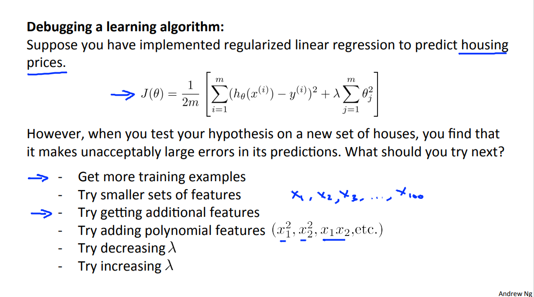
The question is what should you then try mixing in order to improve the learning algorithm?

There are many things that one can think of that could improve the performance of the learning algorithm.

One thing they could try, is to get more training examples. And concretely, you can imagine, maybe, you know, setting up phone surveys, going door to door, to try to get more data on how much different houses sell for.

And the sad thing is I've seen a lot of people spend a lot of time collecting more training examples, thinking oh, if we have twice as much or ten times as much training data, that is certainly going to help, right? But sometimes getting more training data doesn't actually help and in the next few videos we will see why, and we will see how you can avoid spending a lot of time collecting more training data in settings where it is just not going to help.

Other things you might try are to well maybe try a smaller set of features. So if you have some set of features such as x1, x2, x3 and so on, maybe a large number of features. Maybe you want to spend time carefully selecting some small subset of them to prevent overfitting.

Or maybe you need to get additional features. Maybe the current set of features aren't informative enough and you want to collect more data in the sense of getting more features.

And once again this is the sort of project that can scale up the huge projects can you imagine getting phone surveys to find out more houses, or extra land surveys to find out more about the pieces of land and so on, so a huge project. And once again it would be nice to know in advance if this is going to help before we spend a lot of time doing something like this. We can also try adding polynomial features things like x2 square x2 square and product features x1, x2. We can still spend quite a lot of time thinking about that and we can also try other things like decreasing lambda, the regularization parameter or increasing lambda.

Given a menu of options like these, some of which can easily scale up to six month or longer projects.

Unfortunately, the most common method that people use to pick one of these is to go by gut feeling. In which what many people will do is sort of randomly pick one of these options and maybe say, "Oh, lets go and get more training data." And easily spend six months collecting more training data or maybe someone else would rather be saying, "Well, let's go collect a lot more features on these houses in our data set." And I have a lot of times, sadly seen people spend, you know, literally 6 months doing one of these avenues that they have sort of at random only to discover six months later that that really wasn't a promising avenue to pursue.

Fortunately, there is a pretty simple technique that can let you very quickly rule out half of the things on this list as being potentially promising things to pursue. And there is a very simple technique, that if you run, can easily rule out many of these options, and potentially save you a lot of time pursuing something that's just is not going to work.

In the next two videos after this, I'm going to first talk about how to evaluate learning algorithms. And in the next few videos after that, I'm going to talk about these techniques, which are called the machine learning diagnostics.

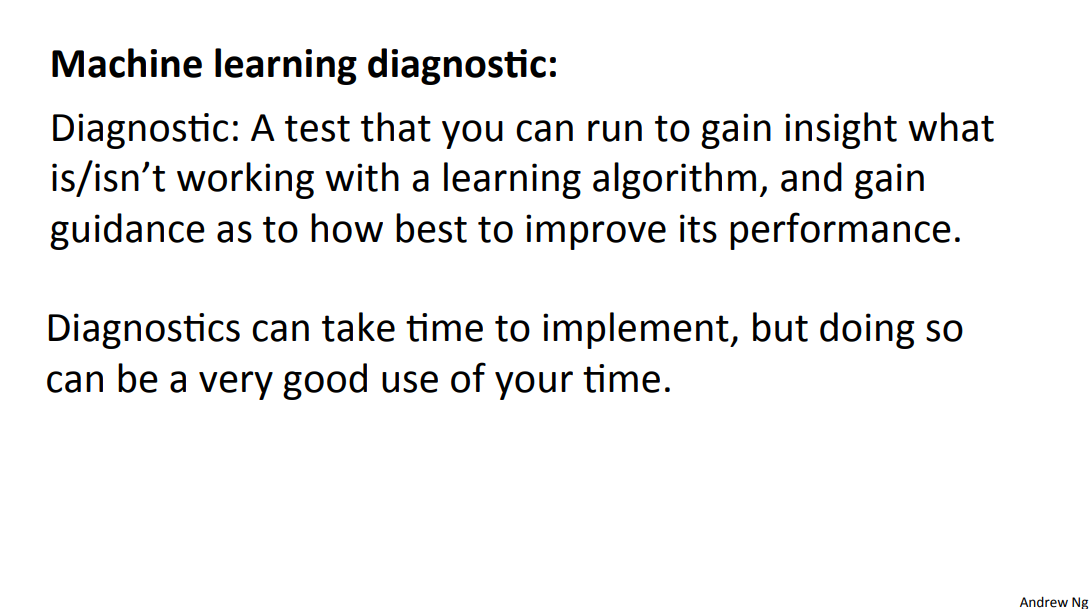
And what a diagnostic is, is a test you can run, to get insight into what is or isn't working with an algorithm, and which will often give you insight as to what are promising things to try to improve a learning algorithm's performance. We'll talk about specific diagnostics later in this video sequence. But I should mention in advance that diagnostics can take time to implement and can sometimes, you know, take quite a lot of time to implement and understand but doing so can be a very good use of your time when you are developing learning algorithms because they can often save you from spending many months pursuing an avenue that you could have found out much earlier just was not going to be fruitful.

So in the next few videos, I'm going to first talk about how evaluate your learning algorithms and after that I'm going to talk about some of these diagnostics which will hopefully let you much more effectively select more of the useful things to try mixing if your goal to improve the machine learning system.

1.2 Evaluating a Hypothesis

Once we have done some trouble shooting for errors in our predictions by:

• Getting more training examples

• Trying smaller sets of features

• Trying additional features

• Trying polynomial features

• Increasing or decreasing λ

We can move on to evaluate our new hypothesis.

A hypothesis may have a low error for the training examples but still be inaccurate (because of overfitting). Thus, to evaluate a hypothesis, given a dataset of training examples, we can split up the data into two sets: a training set and a test set. Typically, the training set consists of 70 % of your data and the test set is the remaining 30 %.

The new procedure using these two sets is then:

1. Learn \(\Theta\) and minimize \(J_{train}(\Theta)\) using the training set

2. Compute the test set error \(J_{test}(\Theta)\)

The test set error:

1. For linear regression:

\[J_{test}(\Theta) = \dfrac{1}{2m_{test}} \sum^{m_{test}}_{i=1}(h_\Theta(x^{(i)}_{test}) - y^{(i)}_{test})^2
\]

1. For classification ~ Misclassification error (aka 0/1 misclassification error):

\[err(h_\Theta(x),y) = \begin{matrix} 1 & \mbox{if } h_\Theta(x) \geq 0.5\ and\ y = 0\ or\ h_\Theta(x) < 0.5\ and\ y = 1\newline 0 & \mbox otherwise \end{matrix}
\]

This gives us a binary 0 or 1 error result based on a misclassification. The average test error for the test set is:

\[\text{Test Error} = \dfrac{1}{m_{test}} \sum^{m_{test}}_{i=1} err(h_\Theta(x^{(i)}_{test}), y^{(i)}_{test})
\]

This gives us the proportion of the test data that was misclassified.

1.3 Model Selection and Train/Validation/Test Sets

Just because a learning algorithm fits a training set well, that does not mean it is a good hypothesis. It could over fit and as a result your predictions on the test set would be poor. The error of your hypothesis as measured on the data set with which you trained the parameters will be lower than the error on any other data set.

Given many models with different polynomial degrees, we can use a systematic approach to identify the 'best' function. In order to choose the model of your hypothesis, you can test each degree of polynomial and look at the error result.

One way to break down our dataset into the three sets is:

• Training set: 60%

• Cross validation set: 20%

• Test set: 20%

We can now calculate three separate error values for the three different sets using the following method:

1. Optimize the parameters in Θ using the training set for each polynomial degree.

2. Find the polynomial degree d with the least error using the cross validation set.

3. Estimate the generalization error using the test set with \(J_{test}(\Theta^{(d)})\), (d = theta from polynomial with lower error);

This way, the degree of the polynomial d has not been trained using the test set.

2 Bias vs. Variance

2.1 Diagnosing Bias vs. Variance

In this section we examine the relationship between the degree of the polynomial d and the underfitting or overfitting of our hypothesis.

• We need to distinguish whether bias or variance is the problem contributing to bad predictions.

• High bias is underfitting and high variance is overfitting. Ideally, we need to find a golden mean between these two.

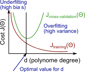
The training error will tend to decrease as we increase the degree d of the polynomial.

At the same time, the cross validation error will tend to decrease as we increase d up to a point, and then it will increase as d is increased, forming a convex curve.

High bias (underfitting): both \(J_{train}(\Theta)\) and \(J_{CV}(\Theta)\) will be high. Also, \(J_{CV}(\Theta) \approx J_{train}(\Theta)\).

High variance (overfitting): \(J_{train}(\Theta)\) will be low and \(J_{CV}(\Theta)\) will be much greater than \(J_{train}(\Theta)\)

The is summarized in the figure below:

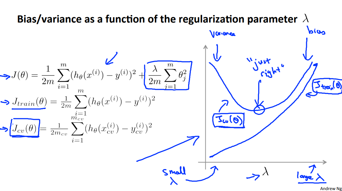
2.2 Regularization and Bias/Variance

Note: [The regularization term below and through out the video should be \(\frac \lambda {2m} \sum _{j=1}^n \theta_j ^2\)]

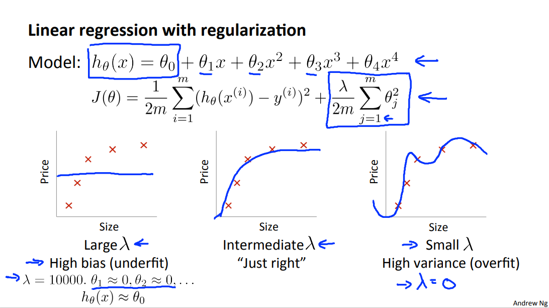
In the figure above, we see that as \(\lambda\) increases, our fit becomes more rigid. On the other hand, as \(\lambda\) approaches 0, we tend to over overfit the data. So how do we choose our parameter \(\lambda\) to get it 'just right' ? In order to choose the model and the regularization term \(\lambda\), we need to:

1. Create a list of lambdas (i.e. λ∈{0,0.01,0.02,0.04,0.08,0.16,0.32,0.64,1.28,2.56,5.12,10.24});

2. Create a set of models with different degrees or any other variants.

3. Iterate through the \(\lambda\)s and for each \(\lambda\) go through all the models to learn some \(\Theta\).

4. Compute the cross validation error using the learned Θ (computed with λ) on the \(J_{CV}(\Theta)\) without regularization or λ = 0.

5. Select the best combo that produces the lowest error on the cross validation set.

6. Using the best combo Θ and λ, apply it on \(J_{test}(\Theta)\) to see if it has a good generalization of the problem.

2.3 Learning Curves

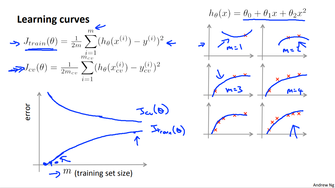
Training an algorithm on a very few number of data points (such as 1, 2 or 3) will easily have 0 errors because we can always find a quadratic curve that touches exactly those number of points. Hence:

• As the training set gets larger, the error for a quadratic function increases.

• The error value will plateau out after a certain m, or training set size.

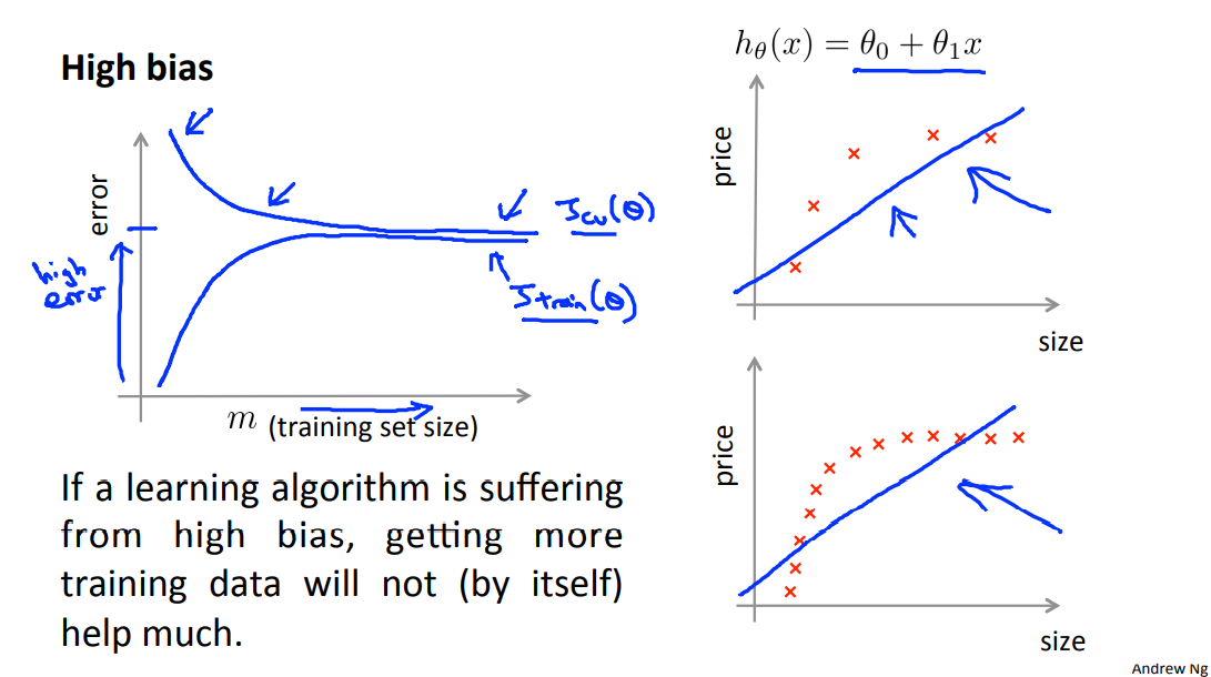
Experiencing high bias:

Low training set size: causes \(J_{train}(\Theta)\) to be low and \(J_{CV}(\Theta)\) to be high.

Large training set size: causes both \(J_{train}(\Theta)\) and \(J_{CV}(\Theta)\) to be high with \(J_{train}(\Theta)\)

If a learning algorithm is suffering from high bias, getting more training data will not (by itself) help much.

Experiencing high variance:

Low training set size: : \(J_{train}(\Theta)\) will be low and \(J_{CV}(\Theta)\) will be high.

Large training set size: \(J_{train}(\Theta)\) increases with training set size and \(J_{CV}(\Theta)\) continues to decrease without leveling off. Also, \(J_{train}(\Theta)\) < \(J_{CV}(\Theta)\).

but the difference between them remains significant.

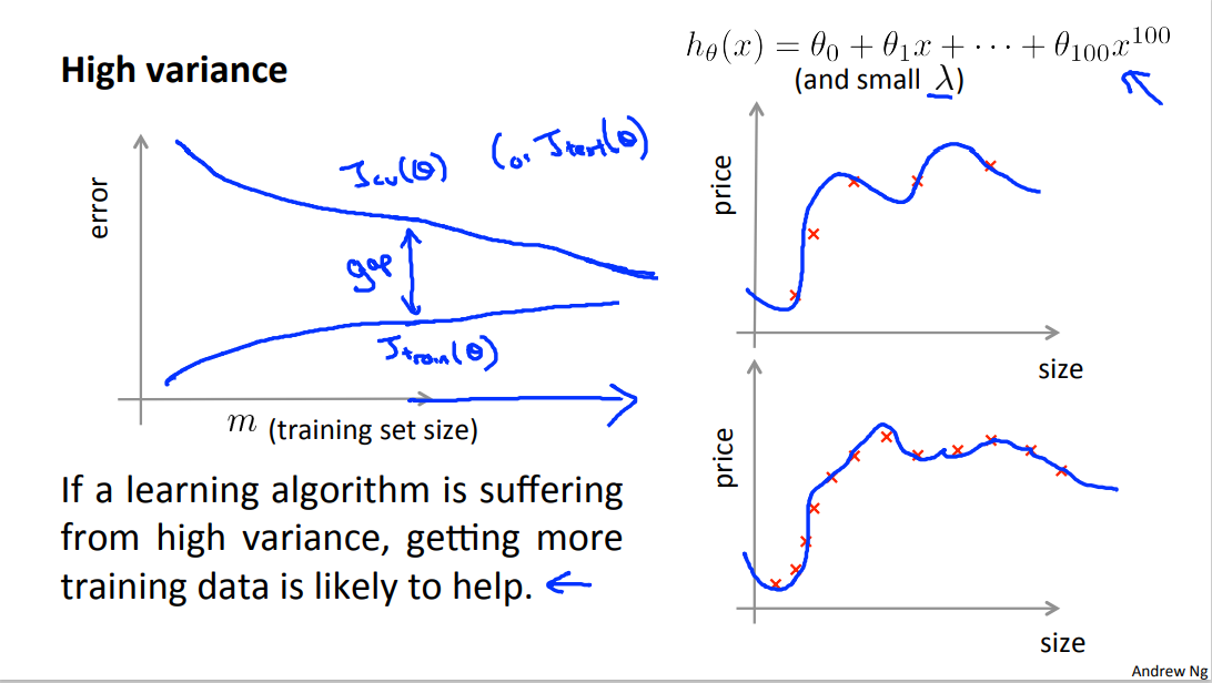
If a learning algorithm is suffering from high variance, getting more training data is likely to help.

学习曲线在数据量为变量时，high bias 的 Jcv 与 Jtrain 两者得非常接近(在数据量非常大的时候，两者可以认为是同质的)，两者都非常大。high variance 的 Jcv 与 Jtrain 两者不太接近，但我觉得还有一条是，Jtrain要小一点。老师所述的情况是两者的差距是 gap, 是一个优质实现的前期状态。不过随着数据量的增加，两者趋于同质，即最后的错误率应该是相近的，但是很小。

做出总结：一旦 Jcv 与 Jtrain，非常相近时，增加数据量不是改进算法的关键因素。

• 可能 01，high bias 算法问题不能很好拟合数据，随着数据量增加数据集趋于同质，在误差上两者会非常接近。

• 可能 02，high variance 算法已经通过巨大的数据量得到了很好的解决。

2.4 Deciding What to Do Next Revisited

Our decision process can be broken down as follows:

• Getting more training examples: Fixes high variance

• Trying smaller sets of features: Fixes high variance

• Adding features: Fixes high bias

• Adding polynomial features: Fixes high bias

• Decreasing λ: Fixes high bias

• Increasing λ: Fixes high variance.

Diagnosing Neural Networks

• A neural network with fewer parameters is prone to underfitting. It is also computationally cheaper.

• A large neural network with more parameters is prone to overfitting. It is also computationally expensive. In this case you can use regularization (increase λ) to address the overfitting.

Using a single hidden layer is a good starting default. You can train your neural network on a number of hidden layers using your cross validation set. You can then select the one that performs best.

Model Complexity Effects:

• Lower-order polynomials (low model complexity) have high bias and low variance. In this case, the model fits poorly consistently.

• Higher-order polynomials (high model complexity) fit the training data extremely well and the test data extremely poorly. These have low bias on the training data, but very high variance.

• In reality, we would want to choose a model somewhere in between, that can generalize well but also fits the data reasonably well.

3 Programming Assignment: Regularized Linear Regression and Bias/Variance

4 Building a Spam classifier

4.1 Prioritizing What to Work On

System Design Example:

Given a data set of emails, we could construct a vector for each email. Each entry in this vector represents a word. The vector normally contains 10,000 to 50,000 entries gathered by finding the most frequently used words in our data set. If a word is to be found in the email, we would assign its respective entry a 1, else if it is not found, that entry would be a 0. Once we have all our x vectors ready, we train our algorithm and finally, we could use it to classify if an email is a spam or not.

So how could you spend your time to improve the accuracy of this classifier?

• Collect lots of data (for example "honeypot" project but doesn't always work)

• Develop sophisticated features

  • for example: using email header data in spam emails
  • for message body, e.g. : should “discount” and “discounts” be treated as the same word? How about “deal” and “Dealer”? Features about punctuation?

• Develop algorithms to process your input in different ways (recognizing misspellings in spam).

  • e.g. m0rtgage, med1cine, w4tches.

It is difficult to tell which of the options will be most helpful.

4.2 Error Analysis

The recommended approach to solving machine learning problems is to:

• Start with a simple algorithm, implement it quickly, and test it early on your cross validation data.

• Plot learning curves to decide if more data, more features, etc. are likely to help.

• Error analysis: Manually examine [ɪɡˈzæmɪn] the examples in cross validation set that your algorithm made errors on. See if you spot any systematic trend in what type of examples it is making errors on.
  
  

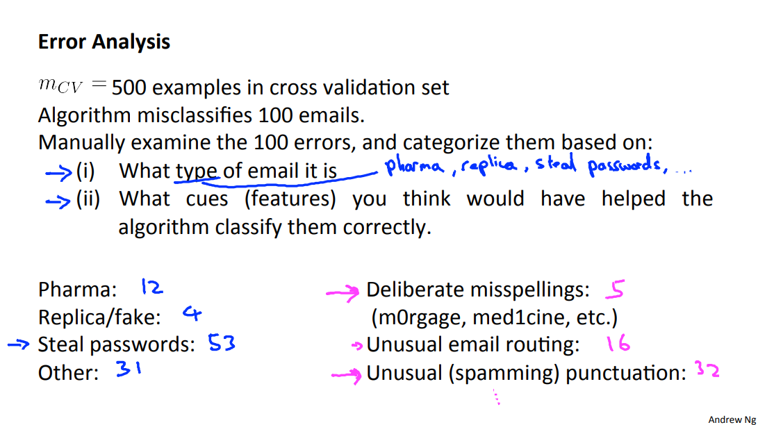
For example, assume that we have 500 emails and our algorithm misclassifies a 100 of them. We could manually analyze the 100 emails and categorize them based on what type of emails they are. We could then try to come up with new cues and features that would help us classify these 100 emails correctly. Hence, if most of our misclassified emails are those which try to steal passwords, then we could find some features that are particular to those emails and add them to our model. We could also see how classifying each word according to its root changes our error rate:

It is very important to get error results as a single, numerical value. Otherwise it is difficult to assess your algorithm's performance. For example if we use stemming(E.g. “Porter stemmer”), which is the process of treating the same word with different forms (fail/failing/failed) as one word (fail).

Error analysis may not be helpful for deciding if this is likely to improve performance. Only solution is to try it and see if it works. And get a 3% error rate instead of 5%, then we should definitely add it to our model. However, if we try to distinguish between upper case and lower case letters and end up getting a 3.2% error rate instead of 3%, then we should avoid using this new feature. Hence, we should try new things, get a numerical value for our error rate, and based on our result decide whether we want to keep the new feature or not.

5 Handing Skewed Data

5.1 Error Metrics for Skewed Classes

For reference:

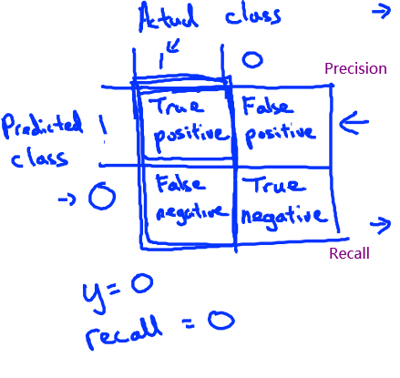
• Accuracy = (true positives + true negatives) / (total examples)

• Precision = (true positives) / (true positives + false positives)

• Recall = (true positives) / (true positives + false negatives)

• \(F_1\) score = (2 * precision * recall) / (precision + recall)

初期理解， precision是 我认为你有cancer 在预测是cancer的情况下。recall是 预测你有cancer 在确实是cancer的情况下. 注意表格中每一列之和对于任意算法都是一致的，因为实际的情况不会随算法而改变。

In the previous video, I talked about error analysis and the importance of having error metrics, that is of having a single real number evaluation metric for your learning algorithm to tell how well it's doing.

In the context of evaluation and of error metrics, there is one important case, where it's particularly tricky to come up with an appropriate error metric, or evaluation metric, for your learning algorithm.

That case is the case of what's called skewed classes. Let me tell you what that means.

Consider the problem of cancer classification, where we have features of medical patients and we want to decide whether or not they have cancer. So this is like the malignant versus benign tumor classification example that we had earlier.

So let's say y equals 1 if the patient has cancer and y equals 0 if they do not. We have trained the progression classifier and let's say we test our classifier on a test set and find that we get 1 percent error. So, we're making 99% correct diagnosis. Seems like a really impressive result, right. We're correct 99% percent of the time.

But now, let's say we find out that only 0.5 percent of patients in our training test sets actually have cancer. So only half a percent of the patients that come through our screening process have cancer. In this case, the 1% error no longer looks so impressive.

And in particular, here's a piece of code, here's actually a piece of non learning code that takes this input of features x and it ignores it. It just sets y equals 0 and always predicts, you know, nobody has cancer and this algorithm would actually get 0.5 percent error. So this is even better than the 1% error that we were getting just now and this is a non learning algorithm that you know, it is just predicting y equals 0 all the time.

So this setting of when the ratio of positive to negative examples is very close to one of two extremes, where, in this case, the number of positive examples is much, much smaller than the number of negative examples because y equals one so rarely, this is what we call the case of skewed classes.

We just have a lot more of examples from one class than from the other class. And by just predicting y equals 0 all the time, or maybe our predicting y equals 1 all the time, an algorithm can do pretty well. So the problem with using classification error or classification accuracy as our evaluation metric is the following.

Let's say you have one joining algorithm that's getting 99.2% accuracy.

So, that's a 0.8% error. Let's say you make a change to your algorithm and you now are getting 99.5% accuracy.

That is 0.5% error.

So, is this an improvement to the algorithm or not? One of the nice things about having a single real number evaluation metric is this helps us to quickly decide if we just need a good change to the algorithm or not. By going from 99.2% accuracy to 99.5% accuracy.

You know, did we just do something useful or did we just replace our code with something that just predicts y equals zero more often? So, if you have very skewed classes it becomes much harder to use just classification accuracy, because you can get very high classification accuracies or very low errors, and it's not always clear if doing so is really improving the quality of your classifier because predicting y equals 0 all the time doesn't seem like a particularly good classifier.

But just predicting y equals 0 more often can bring your error down to, you know, maybe as low as 0.5%. When we're faced with such a skewed classes therefore we would want to come up with a different error metric or a different evaluation metric. One such evaluation metric are what's called precision recall. Let me explain what that is.

Let's say we are evaluating a classifier on the test set. For the examples in the test set the actual class of that example in the test set is going to be either one or zero, right, if there is a binary classification problem.

And what our learning algorithm will do is it will, you know, predict some value for the class and our learning algorithm will predict the value for each example in my test set and the predicted value will also be either one or zero.

So let me draw a two by two table as follows, depending on a full of these entries depending on what was the actual class and what was the predicted class. If we have an example where the actual class is one and the predicted class is one then that's called an example that's a true positive, meaning our algorithm predicted that it's positive and in reality the example is positive. If our learning algorithm predicted that something is negative, class zero, and the actual class is also class zero then that's what's called a true negative. We predicted zero and it actually is zero.

To find the other two boxes, if our learning algorithm predicts that the class is one but the actual class is zero, then that's called a false positive.

So that means our algorithm for the patient is cancer out in reality if the patient does not.

And finally, the last box is a zero, one. That's called a false negative because our algorithm predicted zero, but the actual class was one. And so, we have this little sort of two by two table based on what was the actual class and what was the predicted class.

So here's a different way of evaluating the performance of our algorithm. We're going to compute two numbers.

The first is called precision - and what that says is, of all the patients where we've predicted that they have cancer, what fraction of them actually have cancer?

So let me write this down, the precision of a classifier is the number of true positives divided by the number that we predicted as positive, right?

So of all the patients that we went to those patients and we told them, "We think you have cancer." Of all those patients, what fraction of them actually have cancer? So that's called precision. And another way to write this would be true positives and then in the denominator is the number of predicted positives, and so that would be the sum of the, you know, entries in this first row of the table. So it would be true positives divided by true positives. I'm going to abbreviate positive as POS and then plus false positives, again abbreviating positive using POS.

So that's called precision, and as you can tell high precision would be good. That means that all the patients that we went to and we said, "You know, we're very sorry. We think you have cancer," high precision means that of that group of patients most of them we had actually made accurate predictions on them and they do have cancer.

The second number we're going to compute is called recall, and what recall say is, if all the patients in, let's say, in the test set or the cross-validation set, but if all the patients in the data set that actually have cancer, what fraction of them that we correctly detect as having cancer. So if all the patients have cancer, how many of them did we actually go to them and you know, correctly told them that we think they need treatment.

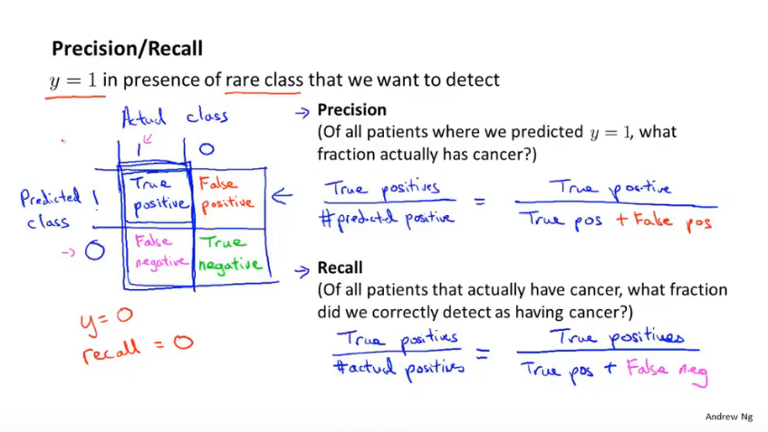
So, writing this down, recall is defined as the number of positives, the number of true positives, meaning the number of people that have cancer and that we correctly predicted have cancer and we take that and divide that by, divide that by the number of actual positives, so this is the right number of actual positives of all the people that do have cancer. What fraction do we directly flag and you know, send the treatment.

So, to rewrite this in a different form, the denominator would be the number of actual positives as you know, is the sum of the entries in this first column over here. And so writing things out differently, this is therefore, the number of true positives, divided by the number of true positives plus the number of false negatives. And so once again, having a high recall would be a good thing.

So by computing precision and recall this will usually give us a better sense of how well our classifier is doing.

And in particular if we have a learning algorithm that predicts y equals zero all the time, if it predicts no one has cancer, then this classifier will have a recall equal to zero, because there won't be any true positives and so that's a quick way for us to recognize that, you know, a classifier that predicts y equals 0 all the time, just isn't a very good classifier. And more generally, even for settings where we have very skewed classes, it's not possible for an algorithm to sort of "cheat" and somehow get a very high precision and a very high recall by doing some simple thing like predicting y equals 0 all the time or predicting y equals 1 all the time. And so we're much more sure that a classifier of a high precision or high recall actually is a good classifier, and this gives us a more useful evaluation metric that is a more direct way to actually understand whether, you know, our algorithm may be doing well.

So one final note in the definition of precision and recall, that we would define precision and recall, usually we use the convention that y is equal to 1, in the presence of the more rare class. So if we are trying to detect. rare conditions such as cancer, hopefully that's a rare condition, precision and recall are defined setting y equals 1, rather than y equals 0, to be sort of that the presence of that rare class that we're trying to detect. And by using precision and recall, we find, what happens is that even if we have very skewed classes, it's not possible for an algorithm to you know, "cheat" and predict y equals 1 all the time, or predict y equals 0 all the time, and get high precision and recall. And in particular, if a classifier is getting high precision and high recall, then we are actually confident that the algorithm has to be doing well, even if we have very skewed classes.

So for the problem of skewed classes precision recall gives us more direct insight into how the learning algorithm is doing and this is often a much better way to evaluate our learning algorithms, than looking at classification error or classification accuracy, when the classes are very skewed.

5.2 Trading Off Precision and Recall

In the last video, we talked about precision and recall as an evaluation metric for classification problems with skewed constants. For many applications, we'll want to somehow control the trade-off between precision and recall. Let me tell you how to do that and also show you some even more effective ways to use precision and recall as an evaluation metric for learning algorithms.

As a reminder, here are the definitions of precision and recall from the previous video.

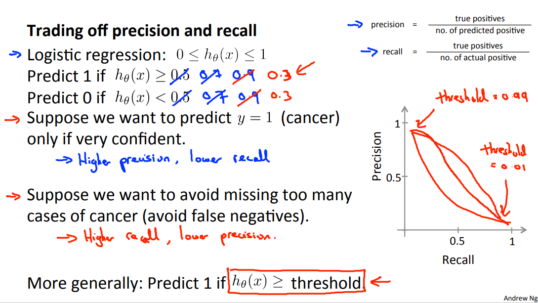
Let's continue our cancer classification example, where y equals 1 if the patient has cancer and y equals 0 otherwise. And let's say we're trained in logistic regression classifier which outputs probability between 0 and 1. So, as usual, we're going to predict 1, y equals 1, if h(x) is greater or equal to 0.5. And predict 0 if the hypothesis outputs a value less than 0.5. And this classifier may give us some value for precision and some value for recall.

But now, suppose we want to predict that the patient has cancer only if we're very confident that they really do. Because if you go to a patient and you tell them that they have cancer, it's going to give them a huge shock. What we give is a seriously bad news, and they may end up going through a pretty painful treatment process and so on. And so maybe we want to tell someone that we think they have cancer only if they are very confident. One way to do this would be to modify the algorithm, so that instead of setting this threshold at 0.5, we might instead say that we will predict that y is equal to 1 only if h(x) is greater or equal to 0.7. So this is like saying, we'll tell someone they have cancer only if we think there's a greater than or equal to, 70% chance that they have cancer.

And, if you do this, then you're predicting someone has cancer only when you're more confident and so you end up with a classifier that has higher precision. Because all of the patients that you're going to and saying, we think you have cancer, although those patients are now ones that you're pretty confident actually have cancer. And so a higher fraction of the patients that you predict have cancer will actually turn out to have cancer because making those predictions only if we're pretty confident.

But in contrast this classifier will have lower recall because now we're going to make predictions, we're going to predict y = 1 on a smaller number of patients. Now, can even take this further. Instead of setting the threshold at 0.7, we can set this at 0.9. Now we'll predict y=1 only if we are more than 90% certain that the patient has cancer. And so, a large fraction of those patients will turn out to have cancer. And so this would be a higher precision classifier will have lower recall because we want to correctly detect that those patients have cancer. Now consider a different example. Suppose we want to avoid missing too many actual cases of cancer, so we want to avoid false negatives. In particular, if a patient actually has cancer, but we fail to tell them that they have cancer then that can be really bad. Because if we tell a patient that they don't have cancer, then they're not going to go for treatment. And if it turns out that they have cancer, but we fail to tell them they have cancer, well, they may not get treated at all. And so that would be a really bad outcome because they die because we told them that they don't have cancer. They fail to get treated, but it turns out they actually have cancer. So, suppose that, when in doubt, we want to predict that y=1. So, when in doubt, we want to predict that they have cancer so that at least they look further into it, and these can get treated in case they do turn out to have cancer.

In this case, rather than setting higher probability threshold, we might instead take this value and instead set it to a lower value. So maybe 0.3 like so, right? And by doing so, we're saying that, you know what, if we think there's more than a 30% chance that they have cancer we better be more conservative and tell them that they may have cancer so that they can seek treatment if necessary.

And in this case what we would have is going to be a higher recall classifier, because we're going to be correctly flagging a higher fraction of all of the patients that actually do have cancer. But we're going to end up with lower precision because a higher fraction of the patients that we said have cancer, a high fraction of them will turn out not to have cancer after all.

And by the way, just as a sider, when I talk about this to other students, I've been told before, it's pretty amazing, some of my students say, is how I can tell the story both ways. Why we might want to have higher precision or higher recall and the story actually seems to work both ways. But I hope the details of the algorithm is true and the more general principle is depending on where you want, whether you want higher precision- lower recall, or higher recall- lower precision. You can end up predicting y=1 when h(x) is greater than some threshold.

And so in general, for most classifiers there is going to be a trade off between precision and recall, and as you vary the value of this threshold that we join here, you can actually plot out some curve that trades off precision and recall. Where a value up here, this would correspond to a very high value of the threshold, maybe threshold equals 0.99. So that's saying, predict y=1 only if we're more than 99% confident, at least 99% probability this one. So that would be a high precision, relatively low recall. Where as the point down here, will correspond to a value of the threshold that's much lower, maybe equal 0.01, meaning, when in doubt at all, predict y=1, and if you do that, you end up with a much lower precision, higher recall classifier. And as you vary the threshold, if you want you can actually trace of a curve for your classifier to see the range of different values you can get for precision recall. And by the way, the precision-recall curve can look like many different shapes. Sometimes it will look like this, sometimes it will look like that. Now there are many different possible shapes for the precision-recall curve, depending on the details of the classifier. So, this raises another interesting question which is, is there a way to choose this threshold automatically?

Or more generally, if we have a few different algorithms or a few different ideas for algorithms, how do we compare different precision recall numbers? Concretely, suppose we have three different learning algorithms. So actually, maybe these are three different learning algorithms, maybe these are the same algorithm but just with different values for the threshold. How do we decide which of these algorithms is best? One of the things we talked about earlier is the importance of a single real number evaluation metric. And that is the idea of having a number that just tells you how well is your classifier doing. But by switching to the precision recall metric we've actually lost that. We now have two real numbers. And so we often, we end up face the situations like if we trying to compare Algorithm 1 and Algorithm 2, we end up asking ourselves, is the precision of 0.5 and a recall of 0.4, was that better or worse than a precision of 0.7 and recall of 0.1? And, if every time you try out a new algorithm you end up having to sit around and think, well, maybe 0.5/0.4 is better than 0.7/0.1, or maybe not, I don't know. If you end up having to sit around and think and make these decisions, that really slows down your decision making process for what changes are useful to incorporate into your algorithm.

Whereas in contrast, if we have a single real number evaluation metric like a number that just tells us is algorithm 1 or is algorithm 2 better, then that helps us to much more quickly decide which algorithm to go with. It helps us as well to much more quickly evaluate different changes that we may be contemplating for an algorithm. So how can we get a single real number evaluation metric?

One natural thing that you might try is to look at the average precision and recall. So, using P and R to denote precision and recall, what you could do is just compute the average and look at what classifier has the highest average value.

But this turns out not to be such a good solution, because similar to the example we had earlier it turns out that if we have a classifier that predicts y=1 all the time, then if you do that you can get a very high recall, but you end up with a very low value of precision. Conversely, if you have a classifier that predicts y equals zero, almost all the time, that is that it predicts y=1 very sparingly, this corresponds to setting a very high threshold using the notation of the previous y. Then you can actually end up with a very high precision with a very low recall. So, the two extremes of either a very high threshold or a very low threshold, neither of that will give a particularly good classifier. And the way we recognize that is by seeing that we end up with a very low precision or a very low recall. And if you just take the average of (P+R)/2 from this example, the average is actually highest for Algorithm 3, even though you can get that sort of performance by predicting y=1 all the time and that's just not a very good classifier, right? You predict y=1 all the time, just normal useful classifier, but all it does is prints out y=1. And so Algorithm 1 or Algorithm 2 would be more useful than Algorithm 3. But in this example, Algorithm 3 has a higher average value of precision recall than Algorithms 1 and 2. So we usually think of this average of precision and recall as not a particularly good way to evaluate our learning algorithm.

In contrast, there's a different way for combining precision and recall. This is called the F Score and it uses that formula. And so in this example, here are the F Scores. And so we would tell from these F Scores, it looks like Algorithm 1 has the highest F Score, Algorithm 2 has the second highest, and Algorithm 3 has the lowest. And so, if we go by the F Score we would pick probably Algorithm 1 over the others.

The F Score, which is also called the F1 Score, is usually written F1 Score that I have here, but often people will just say F Score, either term is used. Is a little bit like taking the average of precision and recall, but it gives the lower value of precision and recall, whichever it is, it gives it a higher weight. And so, you see in the numerator here that the F Score takes a product of precision and recall. And so if either precision is 0 or recall is equal to 0, the F Score will be equal to 0. So in that sense, it kind of combines precision and recall, but for the F Score to be large, both precision and recall have to be pretty large. I should say that there are many different possible formulas for combing precision and recall. This F Score formula is really maybe a, just one out of a much larger number of possibilities, but historically or traditionally this is what people in Machine Learning seem to use. And the term F Score, it doesn't really mean anything, so don't worry about why it's called F Score or F1 Score.

But this usually gives you the effect that you want because if either a precision is zero or recall is zero, this gives you a very low F Score, and so to have a high F Score, you kind of need a precision or recall to be one. And concretely, if P=0 or R=0, then this gives you that the F Score = 0. Whereas a perfect F Score, so if precision equals one and recall equals 1, that will give you an F Score,that's equal to 1 times 1 over 2 times 2, so the F Score will be equal to 1, if you have perfect precision and perfect recall. And intermediate values between 0 and 1, this usually gives a reasonable rank ordering of different classifiers.

So in this video, we talked about the notion of trading off between precision and recall, and how we can vary the threshold that we use to decide whether to predict y=1 or y=0. So it's the threshold that says, do we need to be at least 70% confident or 90% confident, or whatever before we predict y=1. And by varying the threshold, you can control a trade off between precision and recall. We also talked about the F Score, which takes precision and recall, and again, gives you a single real number evaluation metric. And of course, if your goal is to automatically set that threshold to decide what's really y=1 and y=0, one pretty reasonable way to do that would also be to try a range of different values of thresholds. So you try a range of values of thresholds and evaluate these different thresholds on, say, your cross-validation set and then to pick whatever value of threshold gives you the highest F Score on your crossvalidation [INAUDIBLE]. And that be a pretty reasonable way to automatically choose the threshold for your classifier as well.

6 Using Large Data sets

6.1 Data For Machine Learning

In the previous video, we talked about evaluation metrics.

In this video, I'd like to switch tracks a bit and touch on another important aspect of machine learning system design, which will often come up, which is the issue of how much data to train on. Now, in some earlier videos, I had cautioned against blindly going out and just spending lots of time collecting lots of data, because it's only sometimes that that would actually help.

But it turns out that under certain conditions, and I will say in this video what those conditions are, getting a lot of data and training on a certain type of learning algorithm, can be a very effective way to get a learning algorithm to do very good performance.

And this arises often enough that if those conditions hold true for your problem and if you're able to get a lot of data, this could be a very good way to get a very high performance learning algorithm.

So in this video, let's talk more about that. Let me start with a story.

Many, many years ago, two researchers that I know, Michelle Banko and Eric Broule ran the following fascinating study.

They were interested in studying the effect of using different learning algorithms versus trying them out on different training set sciences, they were considering the problem of classifying between confusable words, so for example, in the sentence: for breakfast I ate, should it be to, two or too? Well, for this example, for breakfast I ate two, 2 eggs.

So, this is one example of a set of confusable words and that's a different set. So they took machine learning problems like these, sort of supervised learning problems to try to categorize what is the appropriate word to go into a certain position in an English sentence.

They took a few different learning algorithms which were, you know, sort of considered state of the art back in the day, when they ran the study in 2001, so they took a variance, roughly a variance on logistic regression called the Perceptron. They also took some of their algorithms that were fairly out back then but somewhat less used now so when the algorithm also very similar to which is a regression but different in some ways, much used somewhat less, used not too much right now took what's called a memory based learning algorithm again used somewhat less now. But I'll talk a little bit about that later. And they used a naive based algorithm, which is something they'll actually talk about in this course. The exact algorithms of these details aren't important. Think of this as, you know, just picking four different classification algorithms and really the exact algorithms aren't important.

But what they did was they varied the training set size and tried out these learning algorithms on the range of training set sizes and that's the result they got. And the trends are very clear right first most of these outer rooms give remarkably similar performance. And second, as the training set size increases, on the horizontal axis is the training set size in millions go from you know a hundred thousand up to a thousand million that is a billion training examples. The performance of the algorithms all pretty much monotonically increase and the fact that if you pick any algorithm may be pick a "inferior algorithm" but if you give that "inferior algorithm" more data, then from these examples, it looks like it will most likely beat even a "superior algorithm".

So since this original study which is very influential, there's been a range of many different studies showing similar results that show that many different learning algorithms you know tend to, can sometimes, depending on details, can give pretty similar ranges of performance, but what can really drive performance is you can give the algorithm a ton of training data.

And this is, results like these has led to a saying in machine learning that often in machine learning it's not who has the best algorithm that wins, it's who has the most data So when is this true and when is this not true? Because we have a learning algorithm for which this is true then getting a lot of data is often maybe the best way to ensure that we have an algorithm with very high performance rather than you know, debating worrying about exactly which of these items to use.

Let's try to lay out a set of assumptions under which having a massive training set we think will be able to help.

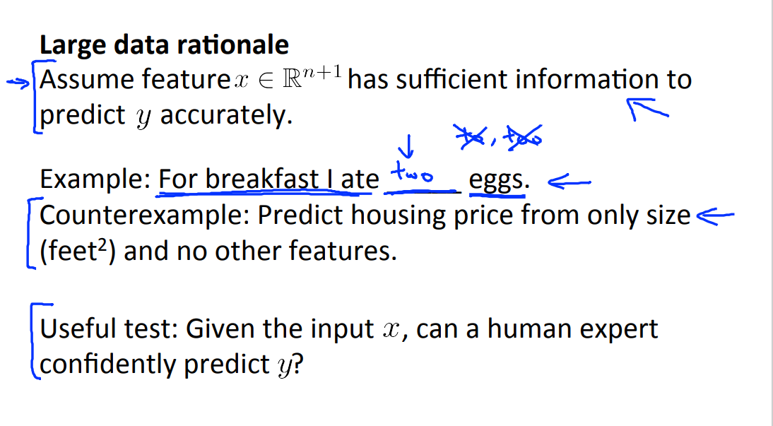
Let's assume that in our machine learning problem, the features x have sufficient information with which we can use to predict y accurately.

For example, if we take the confusable words all of them that we had on the previous slide. Let's say that it features x capture what are the surrounding words around the blank that we're trying to fill in. So the features capture then we want to have, sometimes for breakfast I have blank eggs. Then yeah that is pretty much information to tell me that the word I want in the middle is TWO and that is not word TO and its not the word TOO. So the features capture, you know, one of these surrounding words then that gives me enough information to pretty unambiguously decide what is the label y or in other words what is the word that I should be using to fill in that blank out of this set of three confusable words.

So that's an example what the future x has sufficient information for specific y.

For a counter example. Consider a problem of predicting the price of a house from only the size of the house and from no other features. So if you imagine I tell you that a house is, you know, 500 square feet but I don't give you any other features. I don't tell you that the house is in an expensive part of the city. Or if I don't tell you that the house, the number of rooms in the house, or how nicely furnished the house is, or whether the house is new or old. If I don't tell you anything other than that this is a 500 square foot house, well there's so many other factors that would affect the price of a house other than just the size of a house that if all you know is the size, it's actually very difficult to predict the price accurately.

So that would be a counter example to this assumption that the features have sufficient information to predict the price to the desired level of accuracy. The way I think about testing this assumption, one way I often think about it is, how often I ask myself.

Given the input features x, given the features, given the same information available as well as learning algorithm.

If we were to go to human expert in this domain. Can a human experts actually or can human expert confidently predict the value of y. For this first example if we go to, you know an expert human English speaker. You go to someone that speaks English well, right, then a human expert in English just read most people like you and me will probably we would probably be able to predict what word should go in here, to a good English speaker can predict this well, and so this gives me confidence that x allows us to predict y accurately, but in contrast if we go to an expert in human prices. Like maybe an expert realtor, right, someone who sells houses for a living. If I just tell them the size of a house and I tell them what the price is well even an expert in pricing or selling houses wouldn't be able to tell me and so this is fine that for the housing price example knowing only the size doesn't give me enough information to predict the price of the house. So, let's say, this assumption holds.

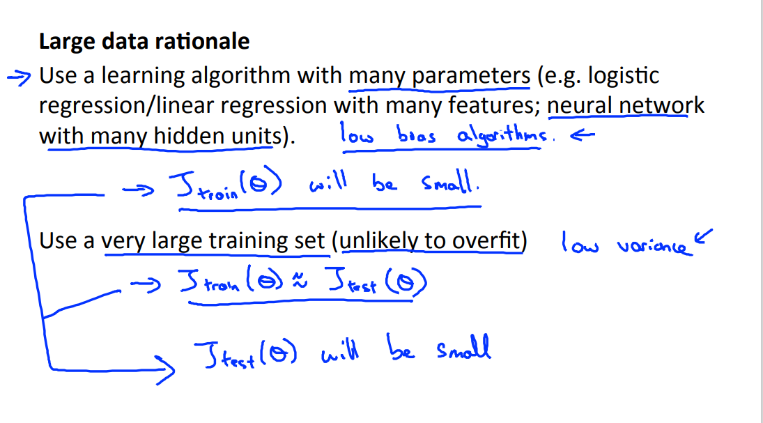
Let's see then, when having a lot of data could help. Suppose the features have enough information to predict the value of y. And let's suppose we use a learning algorithm with a large number of parameters so maybe logistic regression or linear regression with a large number of features. Or one thing that I sometimes do, one thing that I often do actually is using neural network with many hidden units. That would be another learning algorithm with a lot of parameters.

So these are all powerful learning algorithms with a lot of parameters that can fit very complex functions.

So, I'm going to call these, I'm going to think of these as low-bias algorithms because you know we can fit very complex functions and because we have a very powerful learning algorithm, they can fit very complex functions.

Chances are, if we run these algorithms on the data sets, it will be able to fit the training set well, and so hopefully the training error will be slow.

Now let's say, we use a massive, massive training set, in that case, if we have a huge training set, then hopefully even though we have a lot of parameters but if the training set is sort of even much larger than the number of parameters then hopefully these albums will be unlikely to overfit.

Right because we have such a massive training set and by unlikely to overfit what that means is that the training error will hopefully be close to the test error. Finally putting these two together that the train set error is small and the test set error is close to the training error what this two together imply is that hopefully the test set error will also be small.

Another way to think about this is that in order to have a high performance learning algorithm we want it not to have high bias and not to have high variance.

So the bias problem we're going to address by making sure we have a learning algorithm with many parameters and so that gives us a low bias alorithm and by using a very large training set, this ensures that we don't have a variance problem here. So hopefully our algorithm will have no variance and so is by pulling these two together, that we end up with a low bias and a low variance learning algorithm and this allows us to do well on the test set. And fundamentally it's a key ingredients of assuming that the features have enough information and we have a rich class of functions that's why it guarantees low bias, and then it having a massive training set that that's what guarantees more variance.

So this gives us a set of conditions rather hopefully some understanding of what's the sort of problem where if you have a lot of data and you train a learning algorithm with lot of parameters, that might be a good way to give a high performance learning algorithm and really, I think the key test that I often ask myself are first, can a human experts look at the features x and confidently predict the value of y. Because that's sort of a certification that y can be predicted accurately from the features x and second, can we actually get a large training set, and train the learning algorithm with a lot of parameters in the training set and if you can't do both then that's more often give you a very high performance learning algorithm.