Faster RCNN代码解析

1.faster_rcnn_end2end训练

1.1训练入口及配置

def train():
    cfg.GPU_ID = 0
    cfg_file = "../experiments/cfgs/faster_rcnn_end2end.yml"
    cfg_from_file(cfg_file)
    if not False:
        # fix the random seeds (numpy and caffe) for reproducibility
        np.random.seed(cfg.RNG_SEED)
        caffe.set_random_seed(cfg.RNG_SEED)

    # set up caffe
    caffe.set_mode_gpu()
    caffe.set_device(0)

    imdb_name = "voc_2007_trainval"
    imdb, roidb = combined_roidb(imdb_name)
    output_dir = get_output_dir(imdb)
    max_iters = 10000
    pretrained_model = "../data/imagenet_models/ZF.v2.caffemodel"
    solver = "../models/pascal_voc/ZF/faster_rcnn_end2end/solver.prototxt"
    train_net(solver, roidb, output_dir,
              pretrained_model=pretrained_model,
              max_iters=max_iters)

if __name__ == '__main__':
    train()

1.2 数据准备

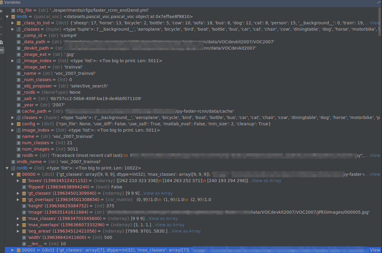
从train_net.py:combined_roidb(imdb_name)处开始，得到的是gt数据集。

输入：“voc_2007_trainval”,  输出：imdb , roidb。 imdb是datasets.pascal_voc.pascal_voc 类，训练图像总数为5011. roidb: 长度为10022,

1.3 训练

跳转到lib/fast_rcnn/train.py:156行。

roidb = filter_roidb(roidb)

由于这里使用的是gt数据集，所以没有过滤任何数据。

sw = SolverWrapper(solver_prototxt, roidb, output_dir,
                       pretrained_model=pretrained_model)

训练中使用了BBOX_REG和BBOX_NORMALIZE_TARGETS，这里需要预计算BBOX的均值和方差。

40行计算bounding-box回归目标：

self.bbox_means, self.bbox_stds = \
                    rdl_roidb.add_bbox_regression_targets(roidb)

跳转到roidb.py的46行，这里对roidb中的每个元素计算‘bbox_targets’. 输入：rois: roidb[im_i]['boxes'], max_overlaps: [1,1,...], max_classes:[9,7,...]

roidb[im_i]['bbox_targets'] = \
                _compute_targets(rois, max_overlaps, max_classes)

_compute_targets()函数返回这个图像中每个推荐框的标签和回归目标(t_i， 见上篇文章http://www.cnblogs.com/benbencoding798/archive/2018/10/26/9856617.html)。不过由于输入的只有真值框，所以得到的回归目标值只有0。接下来是归一化回归目标值。由于gt的值都是0,所以回归目标值也是0。

现在到了lib/fast_rcnn/train.py:44行，建立网络结构。

self.solver = caffe.SGDSolver(solver_prototxt)

models/pascal_voc/ZF/faster_rcnn_end2end/train.prototxt中有4个python层，下面逐一进行调试。

1.4 python层建立

1.4.1 input-data层

数据输入层

layer {
  name: 'input-data'
  type: 'Python'
  top: 'data'
  top: 'im_info' (w, h, im_scales)
  top: 'gt_boxes'
  python_param {
    module: 'roi_data_layer.layer'
    layer: 'RoIDataLayer'
    param_str: "'num_classes': 21"
  }
}

setup()函数执行：
top[0].reshape(1, 3, 600, 1000)
self._name_to_top_map['data'] = 0
top[1].reshape(1, 3)
self._name_to_top_map['im_info'] = 1
top[1].reshape(1, 4)
self._name_to_top_map['gt_boxes'] = 2

在调用lib/roi_data_layer/layer.py中的setup()函数之后，调用reshape(self, bottom, top)函数。

接着调用rpn/__init__.py。

1.4.2 rpn-data层

Assign anchors to ground-truth targets. Produces anchor classification
labels and bounding-box regression targets.

layer {
  name: 'rpn-data'
  type: 'Python'
  bottom: 'rpn_cls_score'
  bottom: 'gt_boxes'
  bottom: 'im_info'
  bottom: 'data'
  top: 'rpn_labels'
  top: 'rpn_bbox_targets'
  top: 'rpn_bbox_inside_weights'
  top: 'rpn_bbox_outside_weights'
  python_param {
    module: 'rpn.anchor_target_layer'
    layer: 'AnchorTargetLayer'
    param_str: "'feat_stride': 16"
  }
}

shape: bottom["rpn_cls_score"]: (img_number, 18, height, width) bottom["gt_boxes"]: (gt_boxes_number, 4), bottom["im_info"]: (img_number, 3), bottom["data"]: (img_number, 3, height, width).

接下来运行rpn/anchor_target_layer.py: setup()。首先看self._anchors

self._anchors = generate_anchors(scales=np.array(anchor_scales))

跳转到rpn/generate_anchors.py:generate_anchors()。这里在rpn/output层特征图的每个位置会生成9个anchors。依我的理解，如果知道一张图片的大小，由于在基本层的卷积之后，图像大小会缩小到原来的1/16,所以每个anchor的位置都能在事先计算出来，并不需要放到rpn.anchor_target_layer计算。下面来看anchors是如何计算的。文中所说，基准的三个anchor size是[(16*8)*(16*8),  (16*16)*(16*16), (16*32)*(16*32)]。在代码中，16是基本大小，[8, 16, 32]是正方形框的伸缩尺度。也就是计算出基本大小上的anchor,乘以伸缩尺度，来得到在原图上的推荐框。

rpn/generate_anchors.py这个文件是用来计算anchor的。

ratio_anchors = _ratio_enum(base_anchor, ratios)

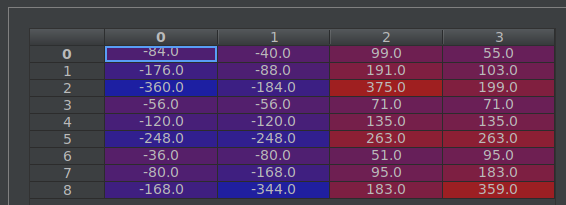
base_anchor是[0,0,15,15],这个代码算出了base_size=16时，三种长宽比例的anchors。计算结果是：[[-3.5, 2, 18.5, 13], [0, 0, 15, 15], [2.5, -3, 12.5, 18]],  直接计算它们的面积，第个和第三个都不会256,这看似计算错误。然而这一个点，看似没有长度，实际上却代表了16个像素。

def _ratio_enum(anchor, ratios):
    """
    Enumerate a set of anchors for each aspect ratio wrt an anchor.
    """

    w, h, x_ctr, y_ctr = _whctrs(anchor)
    size = w * h  # 256
    size_ratios = size / ratios   # [512, 256, 128] 
    ws = np.round(np.sqrt(size_ratios))  # [sqrt(512), sqrt(256), sqrt(128)]
    hs = np.round(ws * ratios)  # [sqrt(512)/2, sqrt(256), 2*sqrt(128)]
    anchors = _mkanchors(ws, hs, x_ctr, y_ctr)
    return anchors

保留根号看，这样是对的，宽和高的乘积都是256, 并且宽高比满足文中条件。

最终9个anchors的结果是：这里需要注意的是中心点的坐标不应该乘以尺度。因为假设计算rpn/output特征图上(0,0)点处的anchors，那么这一点其实代表原图的{0,0,15,15]这一块矩形区域，而中心点正是(7.5,7.5)。9个anchors最终要得到的是在原图的坐标位置，所以中心点是不变的，只是宽度和高度会随尺度缩放。

然后设置输出的shape。以某一图片举例，该图片在rpn/output层size为（39,64）（height, width)。

        # labels （1,1, 9×39, 64）
        top[0].reshape(1, 1, A * height, width)
        # bbox_targets （1,9×4, 39, 64)
        top[1].reshape(1, A * 4, height, width)
        # bbox_inside_weights (1,9*4, 39,64)
        top[2].reshape(1, A * 4, height, width)
        # bbox_outside_weights (1,9*4, 39,64)
        top[3].reshape(1, A * 4, height, width)    

1.4.3 proposal 层

Outputs object detection proposals by applying estimated bounding-box
transformations to a set of regular boxes (called "anchors").    

layer {
  name: 'proposal'
  type: 'Python'
  bottom: 'rpn_cls_prob_reshape'
  bottom: 'rpn_bbox_pred'
  bottom: 'im_info'
  top: 'rpn_rois'
#  top: 'rpn_scores'
  python_param {
    module: 'rpn.proposal_layer'
    layer: 'ProposalLayer'
    param_str: "'feat_stride': 16"
  }
}

ProposalLayer层用于对anchors进行回归矫正得到输出的目标检测框。这层与AnchorTargetLayer相同，也会计算

self._anchors = generate_anchors(scales=np.array(anchor_scales))

# rois blob: holds R regions of interest, each is a 5-tuple
        # (n, x1, y1, x2, y2) specifying an image batch index n and a
        # rectangle (x1, y1, x2, y2)
        top[0].reshape(1, 5)

1.4.4 roi-data 层

Assign object detection proposals to ground-truth targets. Produces proposal
classification labels and bounding-box regression targets.

layer {
  name: 'roi-data'
  type: 'Python'
  bottom: 'rpn_rois'
  bottom: 'gt_boxes'
  top: 'rois'
  top: 'labels'
  top: 'bbox_targets'
  top: 'bbox_inside_weights'
  top: 'bbox_outside_weights'
  python_param {
    module: 'rpn.proposal_target_layer'
    layer: 'ProposalTargetLayer'
    param_str: "'num_classes': 21"
  }
}

shape

# sampled rois (0, x1, y1, x2, y2)
        top[0].reshape(1, 5)
        # labels
        top[1].reshape(1, 1)
        # bbox_targets
        top[2].reshape(1, self._num_classes * 4)
        # bbox_inside_weights
        top[3].reshape(1, self._num_classes * 4)
        # bbox_outside_weights
        top[4].reshape(1, self._num_classes * 4)

1.5 前馈计算

1.5.1 lib/roi_data_layer/layer.py

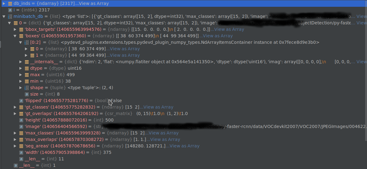
首先是得到当前批次的处理数据。当前设置的__C.TRAIN.IMS_PER_BAT CH=1,

blobs = self._get_next_minibatch()

得到的minibatch_db如下图所示：

得到的blobs如下图所示：

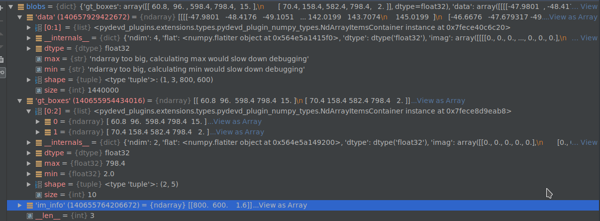
这一层的输入是roidb,输出是‘data’, 'gt_boxes', 'im_info'。

1.5.2 lib/rpn/anchor_target_layer.py

输入：'rpn_cls_score'（bottom_0） , 'gt_boxes', 'im_info', 'data'(bottom_3), 如图所示

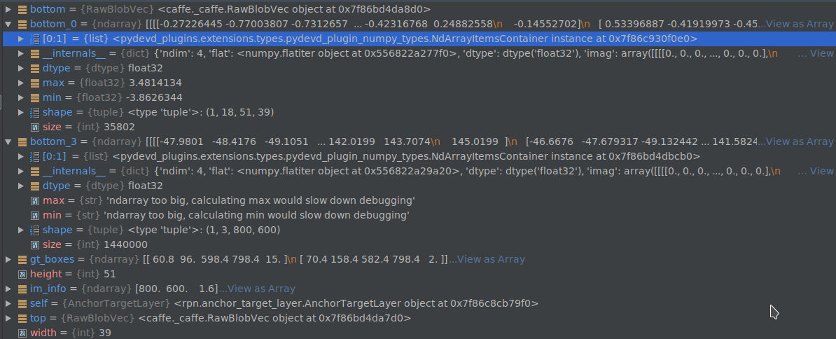
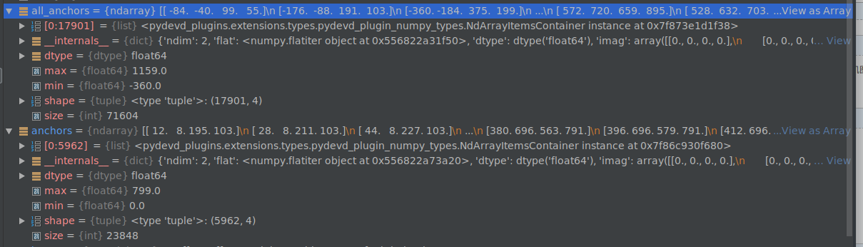
total_anchors 得到卷积之后的特征图的每个anchor在原图中的位置。anchors保留所有不超过原图边界的anchors。下面的anchors都是指这个过滤了与边界相交的。

程序中会计算保留下来的anchors与真值框相关的内容。1.计算每个anchor与每个真值框的IoU, 2.得到每个anchor的最大真值框， 3.得到和每个真值框具有最大IoU的anchor序号（同一个真值框，可能有多个最大值）。4.基于阈值，赋予labels正负标签，当一个anchor和每个真值框的最大IoU小于cfg.TRAIN.RPN_NEGATIVE_OVERLAP=0.3时，赋予负标签， 对与任一真值框具有最大IoU或大于0.7阈值的anchor赋予正标签。5. 对正负样本采样，正样本数最多为128，多余的随机从中选取，负样本用256-正样本数，剩余样本设置为dondon't care。6.计算回归目标。

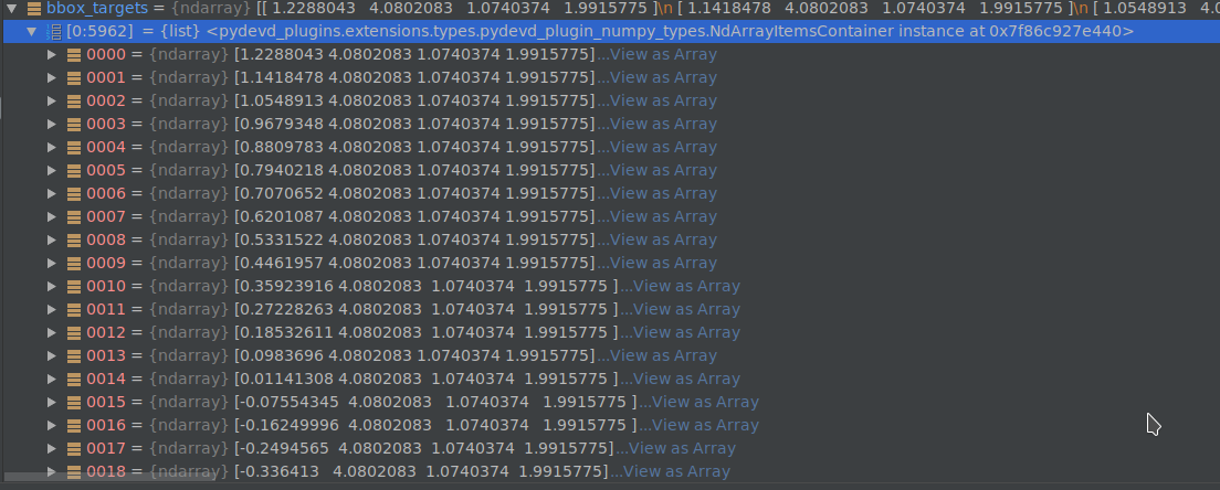
bbox_targets = _compute_targets(anchors, gt_boxes[argmax_overlaps, :])

gt_boxes[argmax_overlaps, :]的数组长度和anchors相同，内容是与anchor面积IoU对应最大的真值框。计算t*（http://www.cnblogs.com/benbencoding798/archive/2018/10/26/9856617.html）

# ex_rois是anchors, gt_rois是与anchors中的每个元素对应的真值框
def bbox_transform(ex_rois, gt_rois):
    ex_widths = ex_rois[:, 2] - ex_rois[:, 0] + 1.0
    ex_heights = ex_rois[:, 3] - ex_rois[:, 1] + 1.0
    ex_ctr_x = ex_rois[:, 0] + 0.5 * ex_widths
    ex_ctr_y = ex_rois[:, 1] + 0.5 * ex_heights

    gt_widths = gt_rois[:, 2] - gt_rois[:, 0] + 1.0
    gt_heights = gt_rois[:, 3] - gt_rois[:, 1] + 1.0
    gt_ctr_x = gt_rois[:, 0] + 0.5 * gt_widths
    gt_ctr_y = gt_rois[:, 1] + 0.5 * gt_heights

    targets_dx = (gt_ctr_x - ex_ctr_x) / ex_widths
    targets_dy = (gt_ctr_y - ex_ctr_y) / ex_heights
    targets_dw = np.log(gt_widths / ex_widths)
    targets_dh = np.log(gt_heights / ex_heights)

    targets = np.vstack(
        (targets_dx, targets_dy, targets_dw, targets_dh)).transpose()
    return targets

得到的bbox_targets如下图。

7.设置权重。bbox_inside_weights，bbox_outside_weights shape为：((len(anchors), 4)

__C.TRAIN.RPN_BBOX_INSIDE_WEIGHTS = (1.0, 1.0, 1.0, 1.0)
#在对应为正样本的anchors列，内部权重给全1

bbox_inside_weights[labels == 1, :] = np.array(cfg.TRAIN.RPN_BBOX_INSIDE_WEIGHTS)

# num_examples为256，就是每张图片的训练样本数
positive_weights = np.ones((1, 4)) * 1.0 / num_examples
negative_weights = np.ones((1, 4)) * 1.0 / num_examples
# 外部权重，采用平均赋值

bbox_outside_weights[labels == 1, :] = positive_weights
bbox_outside_weights[labels == 0, :] = negative_weights

8. 当前集合到原始集合的映射(即从anchors到total_anchors)。labels，bbox_targets, bbox_inside_weights, bbox_outside_weights都做映射。9.对blob[top]的reshape。通过这一层，可以从anchors和真值框 得到每个anchor对应的回归目标值，也就是论文中的t*。并赋值了两个权重矩阵，进而可以在prototxt中计算边框回归的smooth_l1损失值。

1.5.3 lib/rpn/proposal_layer.py

这层的目的就是利用在rpn网络中预测得到的anchors为目标的概率值和回归目标值，计算得到最终的推荐框。这里相当于知道了x_a, t_x,要计算x（见文章https://www.cnblogs.com/benbencoding798/p/9856617.html）

# Algorithm:
        #
        # for each (H, W) location i
        #   generate A anchor boxes centered on cell i
        #   apply predicted bbox deltas at cell i to each of the A anchors
        # clip predicted boxes to image
        # remove predicted boxes with either height or width < threshold
        # sort all (proposal, score) pairs by score from highest to lowest
        # take top pre_nms_topN proposals before NMS
        # apply NMS with threshold 0.7 to remaining proposals
        # take after_nms_topN proposals after NMS
        # return the top proposals (-> RoIs top, scores top)

1.首先得到特征图上每个anchor分类为前景的scores. 2.和上节相同，计算anchors的坐标 3.形状格式化，anchors:(w*h*9,4), bbox_deltas:(w*h*9,4), scores:(w*h*9,1)。3.使用anchors和神经网络回归得到的bbox_deltas计算预测框。4.将越过原图像边框的proposal的相应坐标设置为边界坐标。 5.去除宽度或高度过小的proposal  6. 按proposals预测为前景的分数排序，取前pre_nms_topN个元素。7.应用nms(非极大化抑制)，取前post_nms_topN个元素。8 输出到top的rpn_rois的每个推荐框的第一列元素是每批训练图像的序号索引，由于代码中只实现了单张图片训练实现，所以这列的值都是0，其余四列的值是推荐框的坐标。

输出的rpn_rois shape: (2000, 5)

1.5.4  rpn/proposal_target_layer.py

这里相当于fast rcnn中的数据输入层，因为前面已经得到推荐框了 。现在是计算推荐框和真值框的IoU得到具体的目标标签值（21类），并且计算预测框和真值框的偏移量。

# Sample rois with classification labels and bounding box regressiontargets
        labels, rois, bbox_targets, bbox_inside_weights = _sample_rois(
            all_rois, gt_boxes, fg_rois_per_image,
            rois_per_image, self._num_classes)

这是前馈传播的主要计算内容。all_rois是rois和gt的合集，fg_rois_per_image = 128* 1/4, rois_per_image = 128.

1.首先计算all_rois与gt的IoU。此时all_rois shape: (2002,5), gt_boxes: (2,5), 得到的overlaps shape : (2002,2)

# overlaps: (rois x gt_boxes)
    overlaps = bbox_overlaps(
        np.ascontiguousarray(all_rois[:, 1:5], dtype=np.float),
        np.ascontiguousarray(gt_boxes[:, :4], dtype=np.float))

2.根据overlaps得到all_rois的labels。

labels = gt_boxes[gt_assignment, 4]

3. 根据阈值，选择前景和背景rois和labels.

4.计算rois与对应的gt的偏移量。

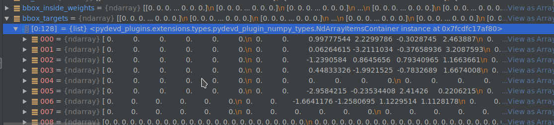
5.将targets映射到84类中，只有前景的targets才进行映射，背景的都是0.对应类的权重是1. bbox_targets shape: (128, 84)