【论文笔记】R-CNN系列之代码实现

代码源码

前情回顾：【论文笔记】R-CNN系列之论文理解

整体架构

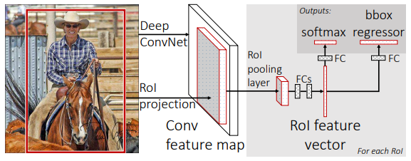
由三部分组成

（1）提取特征的卷积网络extractor

（2）输入特征获得建议框rois的rpn网络

（3）传入rois和特征图，获得分类结果和回归结果的分类网络classifier

伪代码：

class FasterRCNN(nn.Module):
    def __init__(self, ...):
        super(FasterRCNN, self).__init__()
        #   构建特征提取网络
        self.extractor, classifier = decom_vgg16(...)
        #   构建建议框网络
        self.rpn = RegionProposalNetwork(...)
        #   构建分类器网络
        self.head = VGG16RoIHead(..., classifier=classifier)

    def forward(self, x, scale=1.):
        #   计算输入图片的大小
        img_size = x.shape[2:]
        #   利用主干网络提取特征
        base_feature = self.extractor.forward(x)
        #   获得建议框
        _, _, rois, roi_indices, _ = self.rpn.forward(base_feature, img_size, scale)
        #   获得classifier的分类结果和回归结果
        roi_cls_locs, roi_scores = self.head.forward(base_feature, rois, roi_indices, img_size)
        return roi_cls_locs, roi_scores, rois, roi_indices

    def freeze_bn(self):
        for m in self.modules():
            if isinstance(m, nn.BatchNorm2d):
                m.eval()

1.卷积网络提取特征

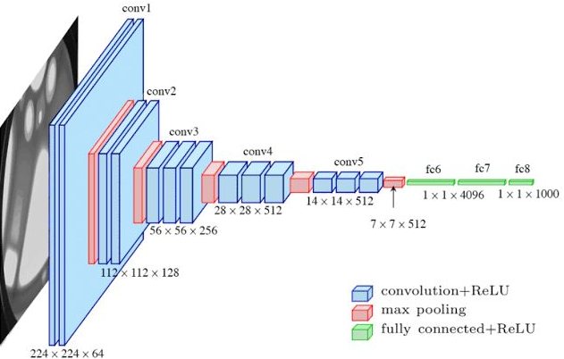
1.1 关于VGG16

代码

import torch
import torch.nn as nn

cfg = [64, 64, 'M', 128, 128, 'M', 256, 256, 256, 'M', 512, 512, 512, 'M', 512, 512, 512, 'M']
'''
假设输入图像为(600, 600, 3)，随着cfg的循环，特征层变化如下：
600,600,3 -> 600,600,64 -> 600,600,64 -> 300,300,64 -> 300,300,128 -> 300,300,128 -> 150,150,128 -> 150,150,256 -> 150,150,256 -> 150,150,256
-> 75,75,256 -> 75,75,512 -> 75,75,512 -> 75,75,512 -> 37,37,512 -> 37,37,512 -> 37,37,512 -> 37,37,512
到cfg结束，我们获得了一个37,37,512的特征层
'''
class VGG16(nn.Module):
    def __init__(self):
        super(VGG16, self).__init__()

        self.feature = make_layers(cfg, batch_norm=False)
        self.avgpool = nn.AdaptiveAvgPool2d((7, 7))    #不管cfg結束后特征层大小是多少，统一变成7*7
        self.classifier = nn.Sequential(
            nn.Linear(7 * 7 * 512, out_features=4096, bias=False),
            nn.ReLU(inplace=True),   # 原地操作更加节省内存
            nn.Linear(in_features=4096, out_features=4096, bias=False),
            nn.ReLU(inplace=True),
            nn.Linear(in_features=4096, out_features=1000, bias=False),
        )

    def forward(self, x):
        x = self.feature(x)
        x = self.avgpool(x)
        x = torch.flatten(x, 1)
        x = self.classifier(x)
        return x

def make_layers(cfg, batch_norm=False):
    input_channels = 3
    layers = []
    for v in cfg:
        if v == 'M':
            layers.append(nn.MaxPool2d(kernel_size=2, stride=2))
        else:
            conv2d = nn.Conv2d(in_channels=input_channels, out_channels=v, kernel_size=3, stride=1, padding=1)
            if batch_norm:
                layers += [conv2d, nn.BatchNorm2d(v), nn.ReLU(inplace=True)]
            else:
                layers += [conv2d, nn.ReLU(inplace=True)]  # layers.append()不能加list
            input_channels = v
    return nn.Sequential(*layers)

input = torch.randn(1, 3, 600, 600)
model = VGG16()
output = model(input)
print(output.shape)

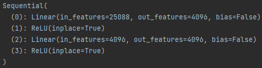
1.2 调整VGG16

• 利用VGG16的特征提取部分作为Faster R-CNN的特征提取网络
• 利用后半部分的全连接网络作为Faster R-CNN的分类网络

def decom_vgg16(pretrained = False):
    model = VGG16()
    feature = list(model.feature)       #转化为list
    classifier = list(model.classifier)
    del classifier[-1] 　　　　　　　　　　# 删去最后的全连接层，如果有dropout层也删掉
    feature = nn.Sequential(*feature)   # 再转为Sequential
    classifier = nn.Sequential(*classifier)
    return feature,classifier

打印一下classifier ：

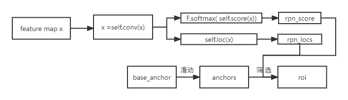
2. RPN生成区域提议

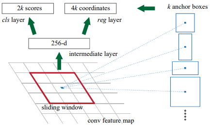
图中的intermediate layer可以用3*3的卷积实现，cls layer和reg layer都可以用1*1的卷积实现。

self.conv1  = nn.Conv2d(in_channels, mid_channels, 3, 1, 1)
self.score  = nn.Conv2d(mid_channels, n_anchor * 2, 1, 1, 0)
self.loc    = nn.Conv2d(mid_channels, n_anchor * 4, 1, 1, 0)

cls layer后接softmax层

reg layer后接筛选层

2.1 anchor

（1）计算出3*3滑动窗口中心点对应原始图像上的中心点

特征图上所有的点，对应原图上固定间隔的点

import matplotlib.pyplot as plt
import numpy as np

if __name__ == "__main__":
    width = 38
    height = 38
    feat_stride = 16
    x = np.arange(0, width * feat_stride, feat_stride)
    y = np.arange(0, height * feat_stride, feat_stride)
    X, Y = np.meshgrid(x, y)
    plt.plot(X, Y,
             color='limegreen',  # 设置颜色为limegreen
             marker='.',  # 设置点类型为圆点
             linestyle='')  # 设置线型为空，也即没有线连接点
    plt.grid(True)
    plt.show()

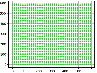
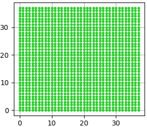
原图                                                                                特征图

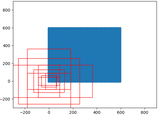
（2）生成anchor box

首先在原图(0,0)位置生成一组（9个）anchor box，然后在原图上滑动（stride=16），得到（38*38*9个）anchor box

#   生成基础的9个先验框
def generate_anchor_base(base_size=16, ratios=[0.5, 1, 2], anchor_scales=[8, 16, 32]):
    anchor_base = np.zeros((len(ratios) * len(anchor_scales), 4), dtype=np.float32)
    for i in range(len(ratios)):
        for j in range(len(anchor_scales)):
            h = base_size * anchor_scales[j] * np.sqrt(ratios[i])
            w = base_size * anchor_scales[j] * np.sqrt(1. / ratios[i])

            index = i * len(anchor_scales) + j
            anchor_base[index, 0] = - h / 2. #框的四个参数分别是左上的（x，y）右下的（x，y）
            anchor_base[index, 1] = - w / 2.
            anchor_base[index, 2] = h / 2.
            anchor_base[index, 3] = w / 2.
    return anchor_base

#   对基础先验框移动对应到所有特征点上(特征点在特征图上是相连的，但对应到原图上间隔feat_stride)
def _enumerate_shifted_anchor(anchor_base, feat_stride, height, width):
    #   计算网格中心点
    shift_x             = np.arange(0, width * feat_stride, feat_stride)
    shift_y             = np.arange(0, height * feat_stride, feat_stride)
    shift_x, shift_y    =np.meshgrid(shift_x, shift_y)
    shift               = np.stack((shift_x.ravel(), shift_y.ravel(), shift_x.ravel(), shift_y.ravel(),), axis=1)
    #   每个网格点上的9个先验框
    A       = anchor_base.shape[0]
    K       = shift.shape[0]
    anchor  = anchor_base.reshape((1, A, 4)) + shift.reshape((K, 1, 4))#应为anchor_base的四个参数都是坐标，所以都要平移
    anchor  = anchor.reshape((K * A, 4)).astype(np.float32)#   所有的先验框
    return anchor    # 38*38*9个

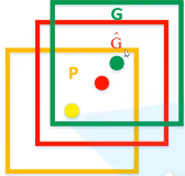
（3）获得预测框

根据rpn得到的k个（dx,dy,dw,dh)，以及上一步得到的k个anchor box的位置（Px,Py,Pw,Ph），可以计算得到预测框的G(Gx,Gy,Gw,Gh)

def loc2bbox(src_bbox, loc):
    if src_bbox.size()[0] == 0:
        return torch.zeros((0, 4), dtype=loc.dtype)
　　# src_bbox就是anchor，四个参数为左上角的坐标和右下角的，所以要转换得到(Px,Py,Pw,Ph)
    src_width   = torch.unsqueeze(src_bbox[:, 2] - src_bbox[:, 0], -1)
    src_height  = torch.unsqueeze(src_bbox[:, 3] - src_bbox[:, 1], -1)
    src_ctr_x   = torch.unsqueeze(src_bbox[:, 0], -1) + 0.5 * src_width
    src_ctr_y   = torch.unsqueeze(src_bbox[:, 1], -1) + 0.5 * src_height
　　# rpn得到的回归参数
    dx          = loc[:, 0::4]
    dy          = loc[:, 1::4]
    dw          = loc[:, 2::4]
    dh          = loc[:, 3::4]
　　# 计算得到预测框的G(Gx,Gy,Gw,Gh)
    ctr_x = dx * src_width + src_ctr_x
    ctr_y = dy * src_height + src_ctr_y
    w = torch.exp(dw) * src_width
    h = torch.exp(dh) * src_height
　　# dst_bbox又是左上角右下角格式
    dst_bbox = torch.zeros_like(loc)
    dst_bbox[:, 0::4] = ctr_x - 0.5 * w
    dst_bbox[:, 1::4] = ctr_y - 0.5 * h
    dst_bbox[:, 2::4] = ctr_x + 0.5 * w
    dst_bbox[:, 3::4] = ctr_y + 0.5 * h

    return dst_bbox

（4）筛选anchor 

# 建议框筛选 （1）出界的不要
roi[:, [0, 2]] = torch.clamp(roi[:, [0, 2]], min=0, max=img_size[1])
roi[:, [1, 3]] = torch.clamp(roi[:, [1, 3]], min=0, max=img_size[0])
# 建议框筛选（2）小于16的不要
min_size = self.min_size * scale
keep = torch.where(((roi[:, 2] - roi[:, 0]) >= min_size) & ((roi[:, 3] - roi[:, 1]) >= min_size))[0]
roi = roi[keep, :]
score = score[keep]
# 建议框筛选（3）按概率选出前n_pre_nms个
order = torch.argsort(score, descending=True)
if n_pre_nms > 0:
    order = order[:n_pre_nms]
roi = roi[order, :]
score = score[order]
# 建议框筛选（4）利用nms选出n_post_nms个
keep = nms(roi, score, self.nms_iou)
keep = keep[:n_post_nms]
roi = roi[keep]

3.分类网络

 分类网络主要分为三部分

（1）ROI pooling layer：将rois转换为固定大小

（2）classifier：VGG16的后半部分全连接层

（3）cls layer 和 loc layer：两个全连接层

伪代码：

class VGG16RoIHead(nn.Module):
    def __init__(self, n_class, roi_size, spatial_scale, classifier):
        super(VGG16RoIHead, self).__init__()
        self.roi = RoIPool((roi_size, roi_size), spatial_scale)
        self.classifier = classifier
        self.cls_loc = nn.Linear(4096, n_class * 4)
        self.score = nn.Linear(4096, n_class)
    def forward(self, x, rois, roi_indices, img_size):
        ...
        # (1) ROI pooling layer
        pool = self.roi(x, indices_and_rois)
        pool = pool.view(pool.size(0), -1)
        # (2) classifier layer
        fc7 = self.classifier(pool)
        # (3) cls layer 和 loc layer
        roi_cls_locs = self.cls_loc(fc7)
        roi_scores = self.score(fc7)
        roi_cls_locs = roi_cls_locs.view(n, -1, roi_cls_locs.size(1))
        roi_scores = roi_scores.view(n, -1, roi_scores.size(1))
        return roi_cls_locs, roi_scores

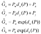
3. 1 ROI pooling layer

将区域提议对应的feature map转换成小的固定大小(H*W)的feature map，不限制输入map的尺寸。

ROI pooling layer的输入有两项：

（1）提取特征的网络的最后一个feature map；

（2）一个表示图片中所有ROI的N*5的矩阵，其中N表示 ROI的数目，5表示图像index和坐标参数(x,y,h,w) 。坐标的参考系不是针对feature map这张图的，而是针对原图的。

...
self.roi = RoIPool((roi_size, roi_size), spatial_scale)
...
pool = self.roi(x, indices_and_rois)# 利用建议框对公用特征层进行截取

(roi_size, roi_size)：执行裁剪后的输出大小（int或Tuple[int，int]），如（高度、宽度）

spatial_scale：将输入坐标映射到框坐标的比例因子。默认值：1.0。

4. 训练

分为几步：

（1）获取公用特征层

（2）利用rpn网络获得调整参数、得分、建议框、先验框

（3）计算损失

4.1 计算建议框网络rpn的回归损失和分类损失

（0）rpn后我们得到rpn_locs, rpn_scores, rois, roi_indices, anchor，其中anchor是先验框，roi是预测框。

（1）为每个先验框anchor找到对应的最大IOU的真实框

    def _calc_ious(self, anchor, bbox):
        #   获得的ious的shape为[num_anchors, num_gt]
        ious = bbox_iou(anchor, bbox)
        if len(bbox)==0:
            return np.zeros(len(anchor), np.int32), np.zeros(len(anchor)), np.zeros(len(bbox))
        #   获得每一个先验框最对应的真实框  [num_anchors, ]
        argmax_ious = ious.argmax(axis=1)
        #   找出每一个先验框最对应的真实框的iou  [num_anchors, ]
        max_ious = np.max(ious, axis=1)
        #   获得每一个真实框最对应的先验框  [num_gt, ]
        gt_argmax_ious = ious.argmax(axis=0)
        #   保证每一个真实框都存在对应的先验框
        for i in range(len(gt_argmax_ious)):
            argmax_ious[gt_argmax_ious[i]] = i
        return argmax_ious, max_ious, gt_argmax_ious

#   argmax_ious为每个先验框对应的最大的真实框的序号         [num_anchors, ]
#   max_ious为每个真实框对应的最大的真实框的iou             [num_anchors, ]
#   gt_argmax_ious为每一个真实框对应的最大的先验框的序号    [num_gt, ]

（2）采样256个anchor计算损失函数，正负样本比为1：1，如果正样本少于128个，用负样本填充。每个ground truth至少对应一个先验框。

我们分配正标签前景给两类anchor：

1）与某个ground truth有最高的IoU重叠的anchor（也许不到0.7）

2）与任意ground truth有大于0.7的IoU交叠的anchor。

我们分配负标签（背景）给与所有ground truth的IoU比率都低于0.3的anchor。

（3）根据每一个先验框最对应的真实框，得到256个真实框bbox的loc  gt_rpn_loc =（dx,dy,dw,dh)

（4）由rpn网络得到的rpn_loc，rpn_score和真实框得到的gt_rpn_loc，gt_rpn_label计算损失

rpn_loc_loss = self._fast_rcnn_loc_loss(rpn_loc, gt_rpn_loc, gt_rpn_label, self.rpn_sigma)
rpn_cls_loss = F.cross_entropy(rpn_score, gt_rpn_label, ignore_index=-1)

4.2 计算Classifier网络的回归损失和分类损失

（0）rpn后我们得到rpn_locs, rpn_scores, rois, roi_indices, anchor，其中anchor是先验框，roi是预测框。

（1）获得每一个建议框roi最对应的真实框

（2）采样n_sample个建议框roi计算损失函数

满足建议框和真实框重合程度大于neg_iou_thresh_high的作为正样本
将正样本的数量限制在self.pos_roi_per_image以内

满足建议框和真实框重合程度小于neg_iou_thresh_high大于neg_iou_thresh_low作为负样本
将正样本的数量和负样本的数量的总和固定成self.n_sample

（3）得到真实框bbox的loc gt_roi_loc =（dx,dy,dw,dh)

（4）由Classifier网络得到的roi_loc，roi_score，和真实框得到的gt_roi_loc，gt_roi_label计算损失

roi_loc_loss = self._fast_rcnn_loc_loss(roi_loc, gt_roi_loc, gt_roi_label.data, self.roi_sigma)
roi_cls_loss = nn.CrossEntropyLoss(roi_score[0], gt_roi_label)

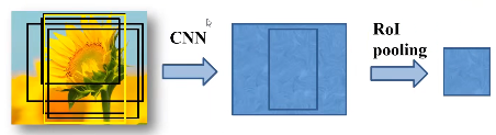
Tip:

上图为4个真实框ground truth，在rpn层中，我们将roi筛选至n_post_nms个（600个）。

在rpn计算的是先验框anchor和真实框bbox的IOU，分类层用的是建议框roi和真实框bbox的IOU

5. 评价指标

5.1计算交并比IOU

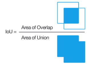
def bbox_iou(bbox_a, bbox_b):
    if bbox_a.shape[1] != 4 or bbox_b.shape[1] != 4:
        print(bbox_a, bbox_b)
        raise IndexError
    tl = np.maximum(bbox_a[:, None, :2], bbox_b[:, :2])
    br = np.minimum(bbox_a[:, None, 2:], bbox_b[:, 2:])
    area_i = np.prod(br - tl, axis=2) * (tl < br).all(axis=2)
    area_a = np.prod(bbox_a[:, 2:] - bbox_a[:, :2], axis=1)
    area_b = np.prod(bbox_b[:, 2:] - bbox_b[:, :2], axis=1)
    return area_i / (area_a[:, None] + area_b - area_i)

5.2 计算AP

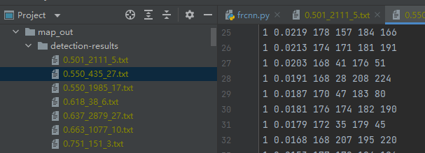
（1）获得预测结果

• 图片送入网络得到预测结果 roi_cls_locs, roi_scores, rois等
• 对建议框进行解码，获得预测框 [ top, left, bottom, right, score, predicted_class ]
• 预测结果写入txt

（2）获得真实框

• 从"VOC2007/Annotations/"+image_id+".xml"中找到xmin，ymin，xmax，ymax
• 写入txt

（3）按照置信度对预测框排序

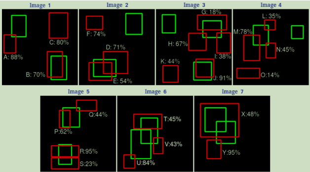
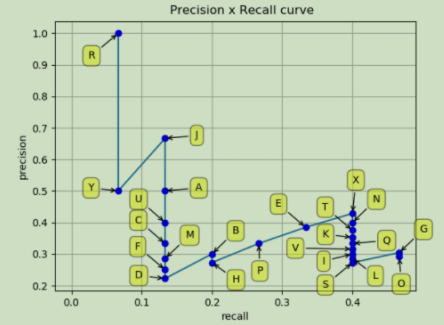
假设一共有7张图片，绿色框是GT（15个），红色框是预测框（24个）并带有置信度。

现在假设IOU=30%，按照置信度排序得到下表。

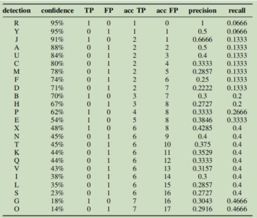
其中TP表示预测正确、FP表示预测错误、acc TP表示从头到该位置累计正确个数、precision表示从头到该位置的精确率、recall表示从头到该位置的召回率。

下图表示的就是从头到尾，依次加入新的样本时，P和R的变化情况：

代码：

• 按照置信度排序

bounding_boxes.sort(key=lambda x:float(x['confidence']), reverse=True)

• 遍历bounding_boxes，计算IOU，大于min_overlap为TP，不然为FP
• 计算precision和recall

for idx, val in enumerate(tp):
rec[idx] = float(tp[idx])/np.maximum(gt_counter_per_class[class_name], 1) # rec=tp/(tp+fn)
　　　　　　　　　　　　　　　　　　　　# gt_counter_per_class 计算每个类有多少个gt，gt的个数=tp+fn
for idx, val in enumerate(tp):
prec[idx] = float(tp[idx]) / np.maximum((fp[idx] + tp[idx]), 1) # prec=tp/(tp+fp)

（4）使精度单调下降，计算PR曲线的面积

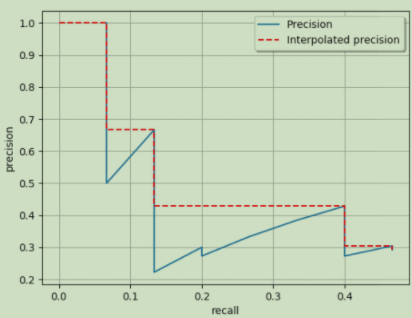
蓝色线就是前面那张PR图，红色虚线的纵坐标是单调减小的，每次减小到右侧蓝线的最高点。APall就是红色虚线下方的面积。

def voc_ap(rec, prec):
    rec.insert(0, 0.0) # insert 0.0 at begining of list
    rec.append(1.0) # insert 1.0 at end of list
    mrec = rec[:]
    prec.insert(0, 0.0) # insert 0.0 at begining of list
    prec.append(0.0) # insert 0.0 at end of list
    mpre = prec[:]
    # 1. 这一部分使精度单调下降
    i_list = []
    for i in range(1, len(mrec)):
        if mrec[i] != mrec[i-1]:
            i_list.append(i) # if it was matlab would be i + 1
    # 2. 平均精度（AP）是曲线下的面积
    ap = 0.0
    for i in i_list:
        ap += ((mrec[i]-mrec[i-1])*mpre[i])
    return ap, mrec, mpre

5.3 mAP指标

如果是多类别目标检测任务，就要使用mean AP(mAP)，其定义为：

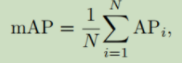
即，对所有的类别进行AP的计算，然后取均值。

AP50指的是IOU的值取50%，AP70同理。

AP@50:5:95指的是IOU的值从50%取到95%，步长为5%，然后算在在这些IOU下的AP的均值。

参考文献：

1. 目标检测01：常用评价指标（AP、AP50、AP@50:5:95、mAP）

2. 睿智的目标检测20——利用mAP计算目标检测精确度

3. Pytorch 搭建自己的Faster-RCNN目标检测平台（视频）

4. 深度学习小技巧-mAP精度概念详解与计算绘制（视频）

5. ROI Pool和ROI Align