逻辑回归代码demo

程序所用文件：https://files.cnblogs.com/files/henuliulei/%E5%9B%9E%E5%BD%92%E5%88%86%E7%B1%BB%E6%95%B0%E6%8D%AE.zip

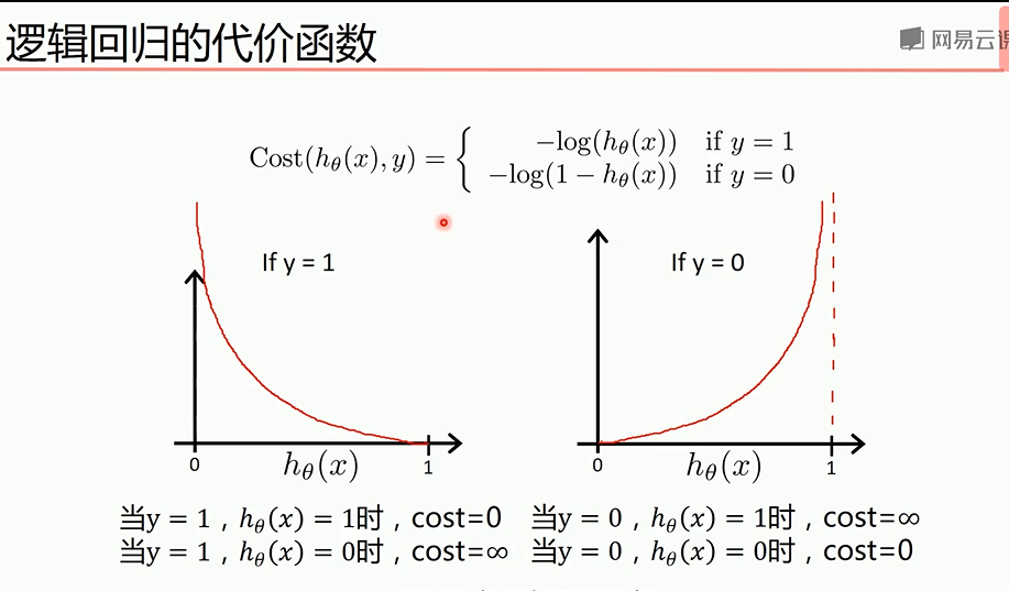
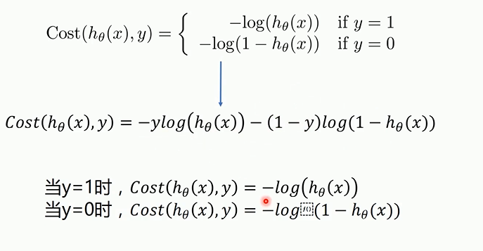
概念

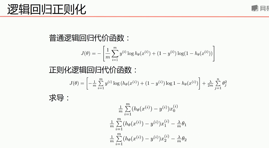
代价函数关于参数的偏导

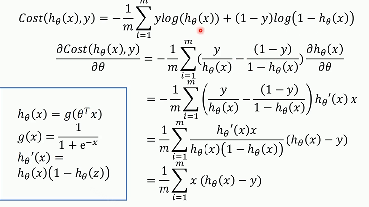
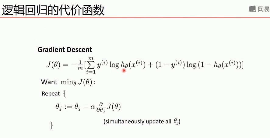
梯度下降法最终的推导公式如下

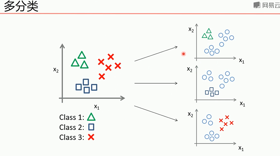
多分类问题可以转为2分类问题

正则化处理可以防止过拟合，下面是正则化后的代价函数和求导后的式子

正确率和召回率F1指标

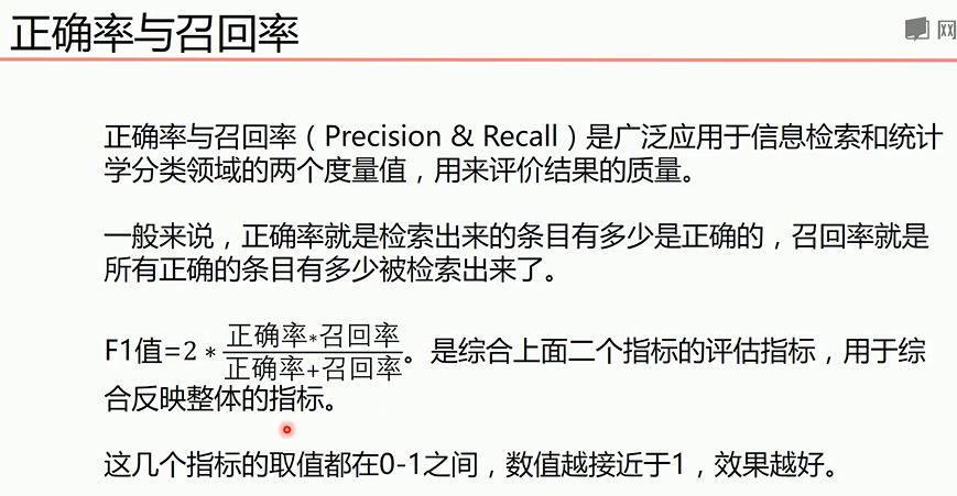
我们希望自己预测的结果希望更准确那么查准率就更高，如果希望更获得更多数量的正确结果，那么查全率更重要，综合考虑可以用F1指标

关于正则化为啥可以防止过拟合的理解

梯度下降法实现线性逻辑回归

 import matplotlib.pyplot as plt
 import numpy as np
 from sklearn.metrics import classification_report#分类
 from sklearn import preprocessing#预测
 # 数据是否需要标准化
 scale = True#True是需要，False是不需要，标准化后效果更好，标准化之前可以画图看出可视化结果
 scale = False
 # 载入数据
 data = np.genfromtxt("LR-testSet.csv", delimiter=",")
 x_data = data[:, :-]
 y_data = data[:, -]

 def plot():
     x0 = []
     x1 = []
     y0 = []
     y1 = []
     # 切分不同类别的数据
     for i in range(len(x_data)):
         if y_data[i] == :
             x0.append(x_data[i, ])
             y0.append(x_data[i, ])
         else:
             x1.append(x_data[i, ])
             y1.append(x_data[i, ])

     # 画图
     scatter0 = plt.scatter(x0, y0, c='b', marker='o')
     scatter1 = plt.scatter(x1, y1, c='r', marker='x')
     # 画图例
     plt.legend(handles=[scatter0, scatter1], labels=['label0', 'label1'], loc='best')

 plot()
 plt.show()
 # 数据处理，添加偏置项
 x_data = data[:,:-]
 y_data = data[:,-,np.newaxis]

 print(np.mat(x_data).shape)
 print(np.mat(y_data).shape)
 # 给样本添加偏置项
 X_data = np.concatenate((np.ones((,)),x_data),axis=)
 print(X_data.shape)

 def sigmoid(x):
     return 1.0 / ( + np.exp(-x))

 def cost(xMat, yMat, ws):
     left = np.multiply(yMat, np.log(sigmoid(xMat * ws)))
     right = np.multiply( - yMat, np.log( - sigmoid(xMat * ws)))
     return np.sum(left + right) / -(len(xMat))

 def gradAscent(xArr, yArr):
     if scale == True:
         xArr = preprocessing.scale(xArr)
     xMat = np.mat(xArr)
     yMat = np.mat(yArr)

     lr = 0.001
     epochs =
     costList = []
     # 计算数据行列数
     # 行代表数据个数，列代表权值个数
     m, n = np.shape(xMat)
     # 初始化权值
     ws = np.mat(np.ones((n, )))

     for i in range(epochs + ):
         # xMat和weights矩阵相乘
         h = sigmoid(xMat * ws)
         # 计算误差
         ws_grad = xMat.T * (h - yMat) / m
         ws = ws - lr * ws_grad

         if i %  == :
             costList.append(cost(xMat, yMat, ws))
     return ws, costList
 # 训练模型，得到权值和cost值的变化
 ws,costList = gradAscent(X_data, y_data)
 print(ws)
 if scale == False:
     # 画图决策边界
     plot()
     x_test = [[-],[]]
     y_test = (-ws[] - x_test*ws[])/ws[]
     plt.plot(x_test, y_test, 'k')
     plt.show()
 # 画图 loss值的变化
 x = np.linspace(, , )
 plt.plot(x, costList, c='r')
 plt.title('Train')
 plt.xlabel('Epochs')
 plt.ylabel('Cost')
 plt.show()
 # 预测
 def predict(x_data, ws):
     if scale == True:
         x_data = preprocessing.scale(x_data)
     xMat = np.mat(x_data)
     ws = np.mat(ws)
     return [ if x >= 0.5 else  for x in sigmoid(xMat*ws)]

 predictions = predict(X_data, ws)

 print(classification_report(y_data, predictions))#计算预测的分

sklearn实现线性逻辑回归

 import matplotlib.pyplot as plt
 import numpy as np
 from sklearn.metrics import classification_report
 from sklearn import preprocessing
 from sklearn import linear_model
 # 数据是否需要标准化
 scale = False
 # 载入数据
 data = np.genfromtxt("LR-testSet.csv", delimiter=",")
 x_data = data[:, :-]
 y_data = data[:, -]

 def plot():
     x0 = []
     x1 = []
     y0 = []
     y1 = []
     # 切分不同类别的数据
     for i in range(len(x_data)):
         if y_data[i] == :
             x0.append(x_data[i, ])
             y0.append(x_data[i, ])
         else:
             x1.append(x_data[i, ])
             y1.append(x_data[i, ])

     # 画图
     scatter0 = plt.scatter(x0, y0, c='b', marker='o')
     scatter1 = plt.scatter(x1, y1, c='r', marker='x')
     # 画图例
     plt.legend(handles=[scatter0, scatter1], labels=['label0', 'label1'], loc='best')

 plot()
 plt.show()
 logistic = linear_model.LogisticRegression()
 logistic.fit(x_data, y_data)
 if scale == False:
     # 画图决策边界
     plot()
     x_test = np.array([[-],[]])
     y_test = (-logistic.intercept_ - x_test*logistic.coef_[][])/logistic.coef_[][]
     plt.plot(x_test, y_test, 'k')
     plt.show()
 predictions = logistic.predict(x_data)

 print(classification_report(y_data, predictions))

梯度下降法实现非线性逻辑回归

 import matplotlib.pyplot as plt
 import numpy as np
 from sklearn.metrics import classification_report
 from sklearn import preprocessing
 from sklearn.preprocessing import PolynomialFeatures
 # 数据是否需要标准化
 scale = False
 # 载入数据
 data = np.genfromtxt("LR-testSet2.txt", delimiter=",")
 x_data = data[:, :-]
 y_data = data[:, -, np.newaxis]

 def plot():
     x0 = []
     x1 = []
     y0 = []
     y1 = []
     # 切分不同类别的数据
     for i in range(len(x_data)):
         if y_data[i] == :
             x0.append(x_data[i, ])
             y0.append(x_data[i, ])
         else:
             x1.append(x_data[i, ])
             y1.append(x_data[i, ])
     # 画图
     scatter0 = plt.scatter(x0, y0, c='b', marker='o')
     scatter1 = plt.scatter(x1, y1, c='r', marker='x')
     # 画图例
     plt.legend(handles=[scatter0, scatter1], labels=['label0', 'label1'], loc='best')

 plot()
 plt.show()
 # 定义多项式回归,degree的值可以调节多项式的特征
 poly_reg  = PolynomialFeatures(degree=)
 # 特征处理
 x_poly = poly_reg.fit_transform(x_data)
 def sigmoid(x):
     return 1.0 / ( + np.exp(-x))

 def cost(xMat, yMat, ws):
     left = np.multiply(yMat, np.log(sigmoid(xMat * ws)))
     right = np.multiply( - yMat, np.log( - sigmoid(xMat * ws)))
     return np.sum(left + right) / -(len(xMat))

 def gradAscent(xArr, yArr):
     if scale == True:
         xArr = preprocessing.scale(xArr)
     xMat = np.mat(xArr)
     yMat = np.mat(yArr)

     lr = 0.03
     epochs =
     costList = []
     # 计算数据列数，有几列就有几个权值
     m, n = np.shape(xMat)
     # 初始化权值
     ws = np.mat(np.ones((n, )))

     for i in range(epochs + ):
         # xMat和weights矩阵相乘
         h = sigmoid(xMat * ws)
         # 计算误差
         ws_grad = xMat.T * (h - yMat) / m
         ws = ws - lr * ws_grad

         if i %  == :
             costList.append(cost(xMat, yMat, ws))
     return ws, costList
 # 训练模型，得到权值和cost值的变化
 ws,costList = gradAscent(x_poly, y_data)
 print(ws)

 # 获取数据值所在的范围
 x_min, x_max = x_data[:, ].min() - , x_data[:, ].max() +
 y_min, y_max = x_data[:, ].min() - , x_data[:, ].max() + 

 # 生成网格矩阵
 xx, yy = np.meshgrid(np.arange(x_min, x_max, 0.02),
                      np.arange(y_min, y_max, 0.02))
 #print(xx.shape)#xx和yy有相同shape，xx的每行相同，总行数取决于yy的范围
 #print(yy.shape)#xx和yy有相同shape，yy的每列相同，总行数取决于xx的范围
 # np.r_按row来组合array，
 # np.c_按colunm来组合array
 # >>> a = np.array([,,])
 # >>> b = np.array([,,])
 # >>> np.r_[a,b]
 # array([, , , , , ])
 # >>> np.c_[a,b]
 # array([[, ],
 #        [, ],
 #        [, ]])
 # >>> np.c_[a,[,,],b]
 # array([[, , ],
 #        [, , ],
 #        [, , ]])
 z = sigmoid(poly_reg.fit_transform(np.c_[xx.ravel(), yy.ravel()]).dot(np.array(ws)))# ravel与flatten类似，多维数据转一维。flatten不会改变原始数据，ravel会改变原始数据
 for i in range(len(z)):
     if z[i] > 0.5:
         z[i] =
     else:
         z[i] =
 print(z)
 z = z.reshape(xx.shape)

 # 等高线图
 cs = plt.contourf(xx, yy, z)
 plot()
 plt.show()
 # 预测
 def predict(x_data, ws):
 #     if scale == True:
 #         x_data = preprocessing.scale(x_data)
     xMat = np.mat(x_data)
     ws = np.mat(ws)
     return [ if x >= 0.5 else  for x in sigmoid(xMat*ws)]

 predictions = predict(x_poly, ws)

 print(classification_report(y_data, predictions))

sklearn实现非线性逻辑回归

 import numpy as np
 import matplotlib.pyplot as plt
 from sklearn import linear_model
 from sklearn.datasets import make_gaussian_quantiles
 from sklearn.preprocessing import PolynomialFeatures
 # 生成2维正态分布，生成的数据按分位数分为两类，500个样本,2个样本特征
 # 可以生成两类或多类数据
 x_data, y_data = make_gaussian_quantiles(n_samples=, n_features=,n_classes=)#生成500个样本，2个特征，2个类别
 plt.scatter(x_data[:, ], x_data[:, ], c=y_data)
 plt.show()
 logistic = linear_model.LogisticRegression()
 logistic.fit(x_data, y_data)
 # 获取数据值所在的范围
 x_min, x_max = x_data[:, ].min() - , x_data[:, ].max() +
 y_min, y_max = x_data[:, ].min() - , x_data[:, ].max() +
 # 生成网格矩阵
 xx, yy = np.meshgrid(np.arange(x_min, x_max, 0.02),
                      np.arange(y_min, y_max, 0.02))
 z = logistic.predict(np.c_[xx.ravel(), yy.ravel()])# ravel与flatten类似，多维数据转一维。flatten不会改变原始数据，ravel会改变原始数据
 z = z.reshape(xx.shape)
 # 等高线图
 cs = plt.contourf(xx, yy, z)
 # 样本散点图
 plt.scatter(x_data[:, ], x_data[:, ], c=y_data)
 plt.show()
 print('score:',logistic.score(x_data,y_data))#使用线性逻辑回归，得分很低

 # 定义多项式回归,degree的值可以调节多项式的特征
 poly_reg  = PolynomialFeatures(degree=)
 # 特征处理
 x_poly = poly_reg.fit_transform(x_data)
 # 定义逻辑回归模型
 logistic = linear_model.LogisticRegression()
 # 训练模型
 logistic.fit(x_poly, y_data)

 # 获取数据值所在的范围
 x_min, x_max = x_data[:, ].min() - , x_data[:, ].max() +
 y_min, y_max = x_data[:, ].min() - , x_data[:, ].max() + 

 # 生成网格矩阵
 xx, yy = np.meshgrid(np.arange(x_min, x_max, 0.02),
                      np.arange(y_min, y_max, 0.02))
 z = logistic.predict(poly_reg.fit_transform(np.c_[xx.ravel(), yy.ravel()]))# ravel与flatten类似，多维数据转一维。flatten不会改变原始数据，ravel会改变原始数据
 z = z.reshape(xx.shape)
 # 等高线图
 cs = plt.contourf(xx, yy, z)
 # 样本散点图
 plt.scatter(x_data[:, ], x_data[:, ], c=y_data)
 plt.show()
 print('score:',logistic.score(x_poly,y_data))#得分很高