壁虎书8 Dimensionality Reduction
many Machine Learning problems involve thousands or even millions of features for each training instance. not only does this make training extremely slow,it can also make it much harder to find a good solution. this problem is often referred to as the curse of dimensionality.
fortunately,in real-world problem,it is often possible to reduce the number of features considerablely,turning an intractable problem into a tractable one. for example,consider the MNIST images,the pixels on the image borders are almost white,so you could completely drop these pixels from the training set without losing much information. Figure 7-6 confirms that these pixels are utterly unimportant for the classification task.
moreover,two neighboring pixels are often highly correlated,if you merge them into a single pixel (e.g., by taking the mean of the two pixels intensities),you will not lose much information.
warning: reducing dimensionality does loss some information,so even though it will speed up training,it may also make your system slightly worse. it also makes your pipelines a bit more complex and thus harder to maintain. so you should first try to train your system with the original data before considering using dimensionality reduction if training is too slow. in some cases,however,reducing the dimensionality of the training data may filter out some noise and unnecessary details and thus result in higher performance (but in general it won't,it will just speed up training).
apart from speeding up training,dimensionality reduction is also extremely useful for data visualization. reducing the number of dimensions down to two (or three) makes it possible to plot a high-dimensional training set on a graph and often gain some important insight by visually detecting patterns,such as clusters.
The Curse of Dimensionality:
we are so used to(习惯) living in three dimension that our intuition fails us when we try to imagine a high-dimensional space. even a basic 4D hypercube is incredibly hard to picture in our mind,let alone a 200-dimensional ellipsoid bent in a 1000-dimensional space.
it turns out that many things behave very differently in high-dimensional space. for example,if you pick a random point in a unit space (a 1 × 1 square),it will have only about a 0.4% (1 - 0.998**2,一个1*1的正方形中,距离边界0.001的一圈) chance of being located less than 0.001 from a border (in other words,it is very unlikely that a random point will be "extreme" along any dimension). but in a 10000-dimensional unit hypercube,this probability is greater than 99.999999%. most points in a high-dimensional hypercube are very close to the border.
here is a more troublesome difference: if you pick two points randomly in a unit square,the distance between these two points will be,on average,roughly 0.52. if you pick two random points in a unit 3D cube,the average distance will be roughly 0.66. in a 1,000,000-dimensional hypercube,it will be about 408.25 (roughly (1,000,000/6)**0.5). this is quite counterintuitive: how can two points be so far apart when they both lie within the same unit hypercube?this fact implies that high-dimensional datasets are at risk of being very sparse: most training instances are likely to be far away from each other. this also means that a new instance will likely be far away from any training instance,making predictions much less reliable than in lower dimensions,since they will be based on much larger extrapolations. in short,the more dimensions the training set has,the greater the risk of overfitting it. 这里的过拟合是从定义上来看的,在测试集上的准确率不如训练集上的准确率。
in theory,one solution to the curse of dimensionality could be to increase the size of the training set to reach a sufficient density of training instances. unfortunately,in practice,the number of training instances required to reach a given density grows exponentially with the number of dimensions. With just 100 features (much less than in the MNIST problem), you would need more training instances than atoms in the observable universe in order for training instances to be within 0.1 of each other on average, assuming they were spread out uniformly across all dimensions.
Main Approaches for Dimensionality Reduction:
Projection
Manifold Learning
Projection:
in most real-world problems,training instances are not spread out uniformly across all dimensions. many features are almost constant,while others are highly correlated (as discussed earlier for MNIST). as a result,all training instances actually lie within (or close to) a much lower-dimensional subspace of the high-dimensional space. in Figure 8-2 you can see a 3D dataset represented by the circles.
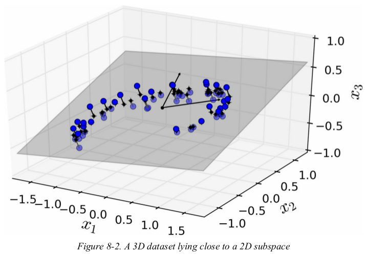
这张图的实现涉及了PCA,稍后回来看。
notice that all training instances lie close to a plane: this is a lower-dimensional(2D) subspace of the high-dimensional(3D) space. now if we project every training instance perpendicularly onto this subspace (as represented by the short lines connecting the instances to the plane),we get the new 2D dataset shown in Figure 8-3. we have just reduced the dataset's dimensionality from 3D to 2D. note that the axes correspond to new features z1 and z2 (the coordinates of the projection on the plane).
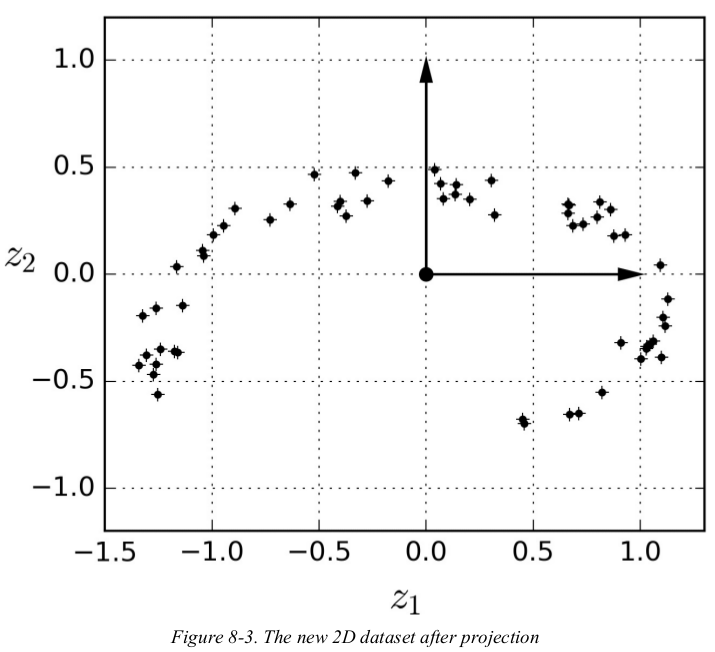
however,projection is not always the best approach to dimensionality reduction. in many cases the subspace may twist and turn,such as the Swiss roll toy dataset represented in Figure 8-4.
 import matplotlib.pyplot as plt

 from mpl_toolkits.mplot3d import Axes3D

 from sklearn.datasets import make_swiss_roll

 X, t = make_swiss_roll(n_samples=1000, noise=0.2, random_state=42)

 axes = [-11.5, 14, -2, 23, -12, 15]

 fig = plt.figure(figsize=(6, 5))

 ax = fig.add_subplot(111, projection='3d')

 ax.scatter(X[:, 0], X[:, 1], X[:, 2], c=t, cmap=plt.cm.hot)

 ax.view_init(10, -70)

 ax.set_xlabel('$x_1$', fontsize=18)

 ax.set_ylabel('$x_2$', fontsize=18)

 ax.set_zlabel('$x_3$', fontsize=18)

 ax.set_xlim(axes[0:2])

 ax.set_ylim(axes[2:4])

 ax.set_zlim(axes[4:6])

 plt.show()
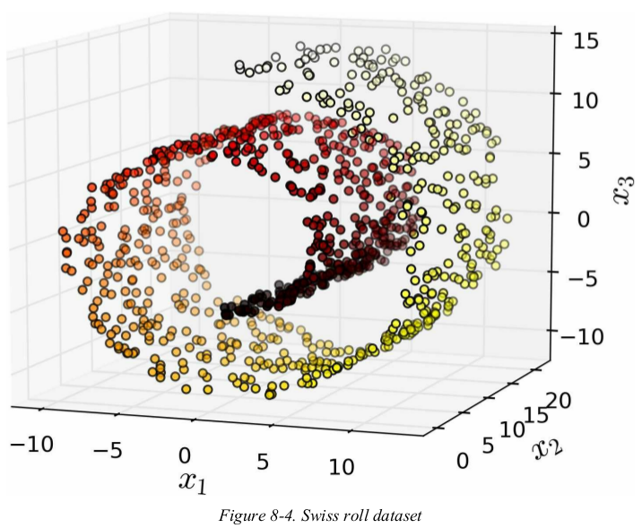
simply projecting onto a plane (e.g., by dropping x3 ) would squash different layers of the Swiss roll together,as shown on the left of Figure 8-5. however,what you really want is to unroll the Swiss roll to obtain the 2D dataset on the right of Figure 8-5.
 import numpy as np

 import matplotlib.pyplot as plt

 from sklearn.datasets import make_swiss_roll

 X, t = make_swiss_roll(n_samples=1000, noise=0.2, random_state=42)

 print(np.min(t), np.max(t))  # 4.756044768712248 14.134506074563456

 axes = [-11.5, 14, -2, 23, -12, 15]

 plt.figure(figsize=(11, 4))

 plt.subplot(121)  # 相当于沿着x3负方向看

 plt.scatter(X[:, 0], X[:, 1], c=t, cmap=plt.cm.hot)

 plt.axis(axes[:4])

 plt.xlabel('$x_1$', fontsize=18)

 plt.ylabel('$x_2$', fontsize=18, rotation=0)

 plt.grid(True)

 plt.subplot(122)  # unroll

 plt.scatter(t, X[:, 1], c=t, cmap=plt.cm.hot)

 plt.axis([4, 15, axes[2], axes[3]])

 plt.xlabel('$z_1$', fontsize=18)

 plt.ylabel('$x_2$', fontsize=18, rotation=0)

 plt.grid(True)

 plt.show()
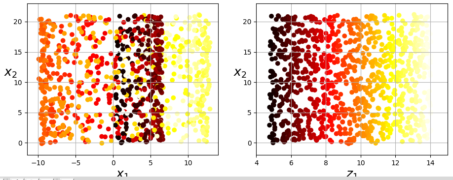
Figure 8-5 Squashing by projecting onto a plane (left) versus unrolling the Swiss roll (right)
Manifold Learning:
the Swiss roll is an example of a 2D manifold. a 2D manifold is a 2D shape that can be bent and twisted in a higher-dimensional space. more generally,a d-dimensional manifold is a part of an n-dimensional space (where d < n) that locally resembles a d-dimensional hyperplane. in the case of the Swiss roll,d = 2 and n = 3: it locally resembles a 2D plane,but it is rolled in the third dimension.
many dimensionality reduction algorithms work by modeling the manifold on which the training instances lie;this is called Manifold Learning. it relies on the manifold assumption,also called the manifold hypothesis,which holds that most real-world high-dimensional datasets lie close to a much lower-dimensional manifold. this assumption is very often empirically observed.
think about the MNIST dataset: all handwritten digit images have some similarities. they are made of connected lines,the borders are white,they are more or less centered,and so on. if you randomly generated images,only a ridiculously tiny fraction of them would look like handwritten digits. in other words,the degrees of freedom available to you if you try to create a digit image are dramatically lower than the degrees of freedom you would have if you were allowed to generate any image you wanted. these constraints tend to squeeze the dataset into a lower-dimensional manifold.
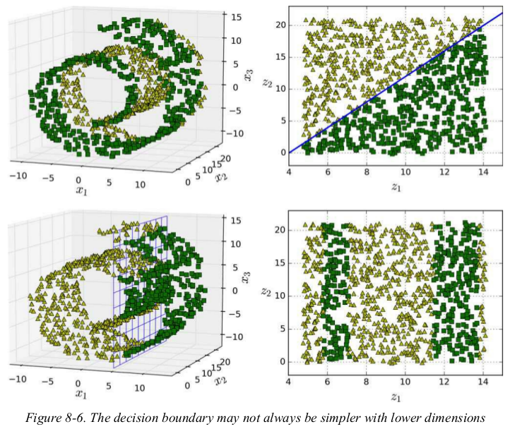
the manifold assumption is often accompanied by another implicit assumption: that the task at hand will be simpler if expressed in the lower-dimensional space of the manifold. For example, in the top row of Figure 8-6 the Swiss roll is split into two classes: in the 3D space (on the left), the decision boundary would be fairly complex, but in the 2D unrolled manifold space (on the right), the decision boundary is a simple straight line.
however,this assumption doesn't always hold. for example,in the bottom row of Figure 8-6,the decision boundary is located at x3 = 5. this decision boundary looks very simple in the original 3D space (a vertical plane),but it looks more complex in the unrolled manifold (a collection of four independent line segments).
in short,if you reduce the dimensionality of your training set before training a model,it will definitely speed up training,but it may not always lead to a better or simpler solution;it all depends on the dataset.
 import numpy as np

 import matplotlib.pyplot as plt

 from mpl_toolkits.mplot3d import Axes3D

 from sklearn.datasets import make_swiss_roll

 X, t = make_swiss_roll(n_samples=1000, noise=0.2, random_state=42)

 # print(np.min(t), np.max(t))  # 4.756044768712248 14.134506074563456

 axes = [-11.5, 14, -2, 23, -12, 15]

 fig = plt.figure(figsize=(8, 8))

 ax = plt.subplot(221, projection='3d')

 positive_class = 2 * (t[:] - 4) > X[:, 1]

 X_pos = X[positive_class]

 X_neg = X[~positive_class]

 ax.view_init(10, -70)

 ax.plot(X_neg[:, 0], X_neg[:, 1], X_neg[:, 2], 'y^')

 ax.plot(X_pos[:, 0], X_pos[:, 1], X_pos[:, 2], 'gs')

 ax.set_xlabel('$x_1$', fontsize=18)

 ax.set_ylabel('$x_2$', fontsize=18)

 ax.set_zlabel('$x_3$', fontsize=18)

 ax.set_xlim(axes[:2])

 ax.set_ylim(axes[2:4])

 ax.set_zlim(axes[4:])

 ax = plt.subplot(222)

 plt.plot(t[positive_class], X[positive_class, 1], 'gs')

 plt.plot(t[~positive_class], X[~positive_class, 1], 'y^')

 plt.plot([4, 15], [0, 22], "b-", linewidth=2)

 plt.axis([4, 15, axes[2], axes[3]])

 plt.xlabel('$z_1$', fontsize=18)

 plt.ylabel('$z_2$', fontsize=18, rotation=0)

 plt.grid(True)

 positive_class = X[:, 0] > 5

 X_pos = X[positive_class]

 X_neg = X[~positive_class]

 ax = plt.subplot(223, projection='3d')

 x2s = np.linspace(axes[2], axes[3], 10)  # 可以控制线图的密度

 x3s = np.linspace(axes[4], axes[5], 10)

 x2, x3 = np.meshgrid(x2s, x3s)

 ax.view_init(10, -70)

 ax.plot(X_neg[:, 0], X_neg[:, 1], X_neg[:, 2], 'y^')

 ax.plot(X_pos[:, 0], X_pos[:, 1], X_pos[:, 2], 'gs')

 ax.plot_wireframe(5, x2, x3, alpha=0.5)

 ax.set_xlabel('$x_1$', fontsize=18)

 ax.set_ylabel('$x_2$', fontsize=18)

 ax.set_zlabel('$x_3$', fontsize=18)

 ax.set_xlim(axes[:2])

 ax.set_ylim(axes[2:4])

 ax.set_zlim(axes[4:])

 ax = plt.subplot(224)

 plt.plot(t[positive_class], X[positive_class, 1], 'gs')

 plt.plot(t[~positive_class], X[~positive_class, 1], 'y^')

 plt.axis([4, 15, axes[2], axes[3]])

 plt.xlabel('$z_1$', fontsize=18)

 plt.ylabel('$z_2$', fontsize=18, rotation=0)

 plt.grid(True)

 plt.show()
PCA:
Preserving the Variance
Principal Components
Projecting Down to d-Dimensions
Using Sckit-Learn
Explained Variance Ratio
Choosing the Right NUmber of Dimensions
PCA for Compression
Incremental PCA
Randomized PCA
Principal Component Analysis (PCA) is by far the most popular dimensionality reduction algorithm. first it identifies the hyperplane that lies closest to the data,and then it projects the data onto it.
Preserving the Variance:
Before you can project the training set onto a lower-dimensional hyperplane, you first need to choose the right hyperplane. For example, a simple 2D dataset is represented on the left of Figure 8-7, along with three different axes (i.e., one-dimensional hyperplanes). On the right is the result of the projection of the dataset onto each of these axes. As you can see, the projection onto the solid line preserves the maximum variance, while the projection onto the dotted line preserves very little variance, and the projection onto the dashed line preserves an intermediate amount of variance.
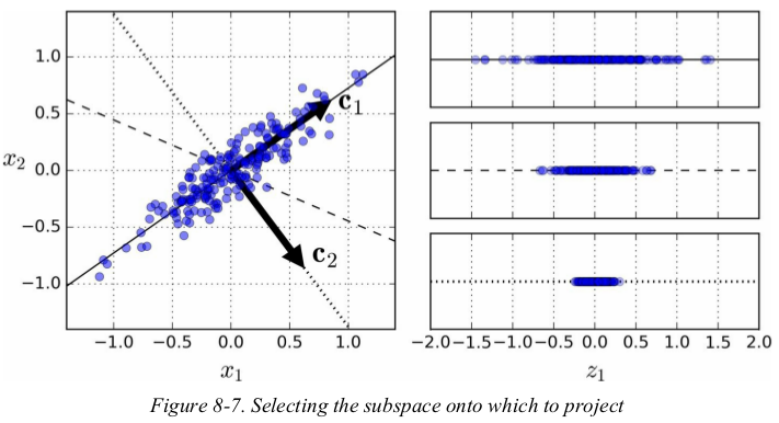
it seems reasonable to select the axis that preserves the maximum amount of variance,as it will most likely lose less information than the other projections. another way to justify this choice is that it is the axis that minimizes the mean squared distance between the original dataset and its projection onto that axis. this is the rather simple idea behind PCA.
Principal Components:
PCA identifies the axis that accounts for the largest amount of variance in the training set. In Figure 8-7, it is the solid line. It also finds a second axis, orthogonal to the first one, that accounts for the largest amount of remaining variance. In this 2D example there is no choice: it is the dotted line. If it were a higher-dimensional dataset, PCA would also find a third axis, orthogonal to both previous axes, and a fourth, a fifth, and so on — as many axes as the number of dimensions in the dataset.
The unit vector that defines the ith axis is called the ith principal component (PC). In Figure 8-7, the 1st PC is c1 and the ith PC is c2 . In Figure 8-2 the first two PCs are represented by the orthogonal arrows in the plane, and the third PC would be orthogonal to the plane (pointing up or down).
Note: the direction of the principal components isn't stable: if you perturb the training set slightly and run PCA again,some of the new PCs may point in the opposite direction of the original PCs. however,they will generally still lie on the same axes. in some cases,a pair of PCs may even rotate or swap,but the plane they define will generally remain the same.
so how can you find the principal components of a training set?there is a standard matrix factorization technique called Singular Value Decomposition (SVD) that can decompose the training set matrix X into the dot product of three matrices U * ∑ * VT,where V contains all the principal components that we are looking for,as shown in Equation 8-1(方程中的应该是V,而不是VT).
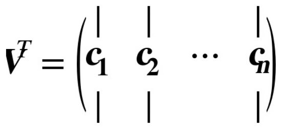 错的!
错的!
the following code uses NumPy's svd() function to obtain all the principal components of the training set,then extracts the first two PCs:
 import numpy as np

 np.random.seed(4)

 m = 60

 w1, w2 = 0.1, 0.3

 noise = 0.1

 angles = np.random.rand(m) * 3 * np.pi / 2 - 0.5

 X = np.empty((m, 3))

 X[:, 0] = np.cos(angles) + np.sin(angles)/2 + noise * np.random.randn(m) / 2

 X[:, 1] = np.sin(angles) * 0.7 + noise * np.random.randn(m) / 2

 X[:, 2] = X[:, 0] * w1 + X[:, 1] * w2 + noise * np.random.randn(m)

 X_centered = X - X.mean(axis=0)

 U, s, Vt = np.linalg.svd(X_centered)

 # print(U.shape, s.shape, Vt.shape)  # (60, 60) (3,) (3, 3)  s是被处理过的

 c1 = Vt.T[:, 0]  # 主成分

 c2 = Vt.T[:, 1]

  # print(c1, c2)  # 降到2D

 m, n = X.shape

 S = np.zeros(X_centered.shape)

 S[:n, :n] = np.diag(s)

 # print(S)

 print(np.allclose(X_centered, U.dot(S).dot(Vt)))  # True
warning: PCA assumes that the dataset is centered around the origin. Scikit-Learn's PCA classes take care of centering the data for you. however,if you implement PCA,don't forget to center the data first.
Projecting Down to d-dimensions:
Once you have identified all the principal components, you can reduce the dimensionality of the dataset down to d dimensions by projecting it onto the hyperplane defined by the first d principal components. Selecting this hyperplane ensures that the projection will preserve as much variance as possible. For example, in Figure 8-2 the 3D dataset is projected down to the 2D plane defined by the first two principal components, preserving a large part of the dataset’s variance. As a result, the 2D projection looks very much like the original 3D dataset.
to project the training set onto the hyperplane,you can simply compute the dot product of the training set matrix X by the matrix Wd,defined as the matrix containing the first d principal components (i.e., the matrix composed of the first d columns of V),as shown in Equation 8-2.

 W2 = Vt.T[:, :2]

 X2D_using_svd = X_centered.dot(W2)

 print(X2D_using_svd)
Using Scikit-Learn:
Scikit-Learn's PCA class implements PCA using SVD decomposition just like we did before,and it automatically takes care of centering the data. 两种方法的结果恰好差一个负号啊。
 import numpy as np

 from sklearn.decomposition import PCA

 X_centered = X - X.mean(axis=0)

 U, s, Vt = np.linalg.svd(X_centered)

 W2 = Vt.T[:, :2]

 X2D_using_svd = X_centered.dot(W2)

 print(X2D_using_svd)

 pca = PCA(n_components=2)

 X2D = pca.fit_transform(X)

 print(np.allclose(X2D_using_svd * (-1), X2D))  # True
after fitting the PCA transformer to the dataset,you can access the principal components using the components_ variable (note that it contains the PCs as horizontal vectors,so the first principal component is equal to pca.components_.T[:, 0]). 两种方法获取结果的方式类似
Explained Variance Ratio: 方差解释率
Another very useful piece of information is the explained variance ratio of each principal component, available via the explained_variance_ratio_ variable. It indicates the proportion of the dataset’s variance that lies along the axis of each principal component. For example, let’s look at the explained variance ratios of the first two components of the 3D dataset represented in Figure 8-2:
print(pca.explained_variance_ratio_) # [0.84248607 0.14631839]
This tells you that 84.2% of the dataset’s variance lies along the first axis, and 14.6% lies along the second axis. This leaves less than 1.2% for the third axis, so it is reasonable to assume that it probably carries little information.
Choosing the Right Number of Dimensions:
Instead of arbitrarily choosing the number of dimensions to reduce down to, it is generally preferable to choose the number of dimensions that add up to a sufficiently large portion of the variance (e.g., 95%). Unless, of course, you are reducing dimensionality for data visualization — in that case you will generally want to reduce the dimensionality down to 2 or 3.
The following code computes PCA without reducing dimensionality, then computes the minimum number of dimensions required to preserve 95% of the training set’s variance:
1 pca = PCA()

2 pca.fit(X)

3 cumsum = np.cumsum(pca.explained_variance_ratio_)

4 print(cumsum)  # [0.84248607 0.98880446 1.        ]

5 d = np.argmax(cumsum >= 0.95) + 1

6 print(d)  # 2
You could then set n_components=d and run PCA again. However, there is a much better option: instead of specifying the number of principal components you want to preserve, you can set n_components to be a float between 0.0 and 1.0 , indicating the ratio of variance you wish to preserve:
 pca = PCA(n_components=0.95)

 X_reduced = pca.fit_transform(X)

 print(pca.n_components_)  #

 print(pca.explained_variance_ratio_)
Yet another option is to plot the explained variance as a function of the number of dimensions (simply plot cumsum; see Figure 8-8). There will usually be an elbow in the curve, where the explained variance stops growing fast. You can think of this as the intrinsic dimensionality of the dataset. In this case, you can see that reducing the dimensionality down to about 100 dimensions wouldn’t lose too much explained variance.

PCA for Compression:
Obviously after dimensionality reduction, the training set takes up much less space. For example, try applying PCA to the MNIST dataset while preserving 95% of its variance. You should find that each instance will have just over 150 features, instead of the original 784 features. So while most of the variance is preserved, the dataset is now less than 20% of its original size! This is a reasonable compression ratio, and you can see how this can speed up a classification algorithm (such as an SVM classifier) tremendously.
It is also possible to decompress the reduced dataset back to 784 dimensions by applying the inverse transformation of the PCA projection. Of course this won’t give you back the original data, since the projection lost a bit of information (within the 5% variance that was dropped), but it will likely be quite close to the original data. The mean squared distance between the original data and the reconstructed data (compressed and then decompressed) is called the reconstruction error. For example, the following code compresses the MNIST dataset down to 154 dimensions, then uses the inverse_transform() method to decompress it back to 784 dimensions.
 pca = PCA(n_components=154)

 X_reduced = pca.fit_transform(X_train)

 print(X_reduced.shape)  # (52500, 154)

 X_recovered = pca.inverse_transform(X_reduced)

 print(X_recovered.shape)  # (52500, 784)
Figure 8-9 shows a few digits from the original training set (on the left), and the corresponding digits after compression and decompression. You can see that there is a slight image quality loss, but the digits are still mostly intact.
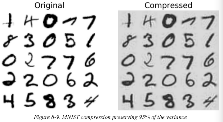 右图是recover之后的
the Equation of the inverse transformation is shown in shown in Equation 8-3.

Incremental PCA:
One problem with the preceding implementation of PCA is that it requires the whole training set to fit in memory in order for the SVD algorithm to run. Fortunately, Incremental PCA (IPCA) algorithms have been developed: you can split the training set into mini-batches and feed an IPCA algorithm one mini-batch at a time. This is useful for large training sets, and also to apply PCA online.
The following code splits the MNIST dataset into 100 mini-batches (using NumPy’s array_split() function) and feeds them to Scikit-Learn’s IncrementalPCA class to reduce the dimensionality of the MNIST dataset down to 154 dimensions (just like before). Note that you must call the partial_fit() method with each mini-batch rather than the fit() method with the whole training set:
 n_batches = 100

 inc_pca = IncrementalPCA(n_components=154)

 for X_batch in np.array_split(X_train, n_batches):

     inc_pca.partial_fit(X_batch)

 X_reduced = inc_pca.transform(X_train)

 print(X_reduced.shape)  # (52500, 154)
Alternatively, you can use NumPy’s memmap class, which allows you to manipulate a large array stored in a binary file on disk as if it were entirely in memory; the class loads only the data it needs in memory, when it needs it. Since the IncrementalPCA class uses only a small part of the array at any given time, the memory usage remains under control. This makes it possible to call the usual fit() method, as you can see in the following code:
 X_mm = np.memmap(filename='fn', dtype='float32', mode='readonly', shape=(m, n))

 batch_size = m // b_batches

 inc_pca = IncrementalPCA(n_components=154, batch_size=batch_size)

 inc_pca.fit(X_mm)
Randomized PCA:
Scikit-Learn offers yet another option to perform PCA, called Randomized PCA. This is a stochastic algorithm that quickly finds an approximation of the first d principal components. Its computational complexity is O(m × d2) + O(d3), instead of O(m × n2) + O(n3), so it is dramatically faster than the previous algorithms when d is much smaller than n.
 rnd_pca = PCA(n_components=154, svd_solver='randomized')

 X_reduced = rnd_pca.fit_transform(X_train)

 print(X_reduced.shape)  # (52500, 154)
Kernel PCA:
Selecting a Kernel and Tuning Hyperparameters
In Chapter 5 we discussed the kernel trick, a mathematical technique that implicitly maps instances into a very high-dimensional space (called the feature space), enabling nonlinear classification and regression with Support Vector Machines. Recall that a linear decision boundary in the high-dimensional feature space corresponds to a complex nonlinear decision boundary in the original space.
It turns out that the same trick can be applied to PCA, making it possible to perform complex nonlinear projections for dimensionality reduction. This is called Kernel PCA (kPCA). It is often good at preserving clusters of instances after projection, or sometimes even unrolling datasets that lie close to a twisted manifold.
For example, the following code uses Scikit-Learn’s KernelPCA class to perform kPCA with an RBF kernel:
 from sklearn.datasets import make_swiss_roll

 from sklearn.decomposition import KernelPCA

 X, t = make_swiss_roll(n_samples=1000, noise=0.2, random_state=42)

 rbf_pca = KernelPCA(n_components=2, kernel='rbf', gamma=0.04)

 X_reduced = rbf_pca.fit_transform(X)

 print(X_reduced.shape)  # (1000, 2)
Figure 8-10 shows the Swiss roll, reduced to two dimensions using a linear kernel (equivalent to simply using the PCA class), an RBF kernel, and a sigmoid kernel (Logistic).
 import matplotlib.pyplot as plt

 from sklearn.datasets import make_swiss_roll

 from sklearn.decomposition import KernelPCA

 X, t = make_swiss_roll(n_samples=1000, noise=0.2, random_state=42)

 y = t > 6.9

 lin_pca = KernelPCA(n_components=2, kernel='linear', fit_inverse_transform=True)

 rbf_pca = KernelPCA(n_components=2, kernel='rbf', gamma=0.0433, fit_inverse_transform=True)

 sig_pca = KernelPCA(n_components=2, kernel='sigmoid', gamma=0.001, coef0=1, fit_inverse_transform=True)

 plt.figure(figsize=(11, 4))

 for subplot, pca, title in ((131, lin_pca, 'Linear kernel'), (132, rbf_pca, 'RBF kernel, $\gamma = 0.04$'), (133, sig_pca, 'Sigmoid kernel, $\gamma=10^{-3}, r=1$')):

     X_reduced = pca.fit_transform(X)

     plt.subplot(subplot)

     plt.title(title)

     plt.scatter(X_reduced[:, 0], X_reduced[:, 1], c=t, cmap=plt.cm.hot)

     plt.xlabel("$z_1$", fontsize=18)

     if subplot == 131:

         plt.ylabel("$z_2$", fontsize=18, rotation=0)

     plt.grid(True)

 plt.show()
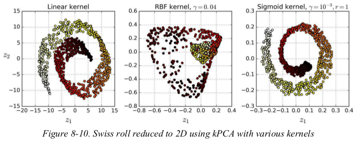
因为主成分方向的原因,图可能不太一致,但形状是一样的。
Selecting a Kernel and Tuning Hyperparameters:
As kPCA is an unsupervised learning algorithm, there is no obvious performance measure to help you select the best kernel and hyperparameter values. However, dimensionality reduction is often a preparation step for a supervised learning task (e.g., classification), so you can simply use grid search to select the kernel and hyperparameters that lead to the best performance on that task.
For example, the following code creates a two-step pipeline, first reducing dimensionality to two dimensions using kPCA, then applying Logistic Regression for classification. Then it uses GridSearchCV to find the best kernel and gamma value for kPCA in order to get the best classification accuracy at the end of the pipeline:
 from sklearn.datasets import make_swiss_roll

 from sklearn.decomposition import KernelPCA

 from sklearn.model_selection import GridSearchCV

 from sklearn.linear_model import LogisticRegression

 from sklearn.pipeline import Pipeline

 X, t = make_swiss_roll(n_samples=1000, noise=0.2, random_state=42)

 y = t > 6.9

 clf = Pipeline([

     ('kpca', KernelPCA(n_components=2)),

     ('log_reg', LogisticRegression(solver='liblinear'))  # 查看solver支持哪些类型,可以随意输入,然后查看报错信息。

 ])

 param_gird = [{

     'kpca__gamma': np.linspace(0.03, 0.05, 10),  # 注意是两个下划线

     'kpca__kernel': ['rbf', 'sigmoid']

 }]

 # If no scoring is specified, the estimator passed should have a 'score' method.

 grid_search = GridSearchCV(clf, param_gird, cv=3)

 grid_search.fit(X, y)

 print(grid_search.best_params_)

 # {'kpca__kernel': 'rbf', 'kpca__gamma': 0.043333333333333335}
Another approach, this time entirely unsupervised, is to select the kernel and hyperparameters that yield the lowest reconstruction error. However, reconstruction is not as easy as with linear PCA. Here’s why. Figure 8-11 shows the original Swiss roll 3D dataset (top left), and the resulting 2D dataset after kPCA is applied using an RBF kernel (top right). Thanks to the kernel trick, this is mathematically equivalent to mapping the training set to an infinite-dimensional feature space (bottom right) using the feature map φ, then projecting the transformed training set down to 2D using linear PCA.
Notice that if we could invert the linear PCA step for a given instance in the reduced space, the reconstructed point would lie in feature space, not in the original space (e.g., like the one represented by an x in the diagram). Since the feature space is infinite-dimensional, we cannot compute the reconstructed point, and therefore we cannot compute the true reconstruction error. Fortunately, it is possible to find a point in the original space that would map close to the reconstructed point. This is called the reconstruction pre-image. Once you have this pre-image, you can measure its squared distance to the original instance. You can then select the kernel and hyperparameters that minimize this reconstruction pre-image error. 这一坨是啥子嘛??今天心好乱...
You may be wondering how to perform this reconstruction. One solution is to train a supervised regression model, with the projected instances as the training set and the original instances as the targets. Scikit-Learn will do this automatically if you set fit_inverse_transform=True, as shown in the following code:
By default, fit_inverse_transform=False and KernelPCA has no inverse_transform() method. This method only gets created when you set fit_inverse_transform=True.
 from sklearn.datasets import make_swiss_roll

 from sklearn.decomposition import KernelPCA

 from sklearn.metrics import mean_squared_error

 X, t = make_swiss_roll(n_samples=1000, noise=0.2, random_state=42)

 y = t > 6.9

 rbf_pca = KernelPCA(n_components=2, kernel='rbf', gamma=0.043, fit_inverse_transform=True)

 X_reduced = rbf_pca.fit_transform(X)

 X_preimage = rbf_pca.inverse_transform(X_reduced)

 print(mean_squared_error(X, X_preimage))  # 32.70536352954476
Now you can use grid search with cross-validation to find the kernel and hyperparameters that minimize this pre-image reconstruction error. 额(⊙o⊙)…??
LLE:
Locally Linear Embedding (LLE) is another very powerful nonlinear dimensionality reduction (NLDR) technique. It is a Manifold Learning technique that does not rely on projections like the previous algorithms. In a nutshell, LLE works by first measuring how each training instance linearly relates to its closest neighbors (c.n.), and then looking for a low-dimensional representation of the training set where these local relationships are best preserved (more details shortly). This makes it particularly good at unrolling twisted manifolds, especially when there is not too much noise.
For example, the following code uses Scikit-Learn’s LocallyLinearEmbedding class to unroll the Swiss roll. The resulting 2D dataset is shown in Figure 8-12. As you can see, the Swiss roll is completely unrolled and the distances between instances are locally well preserved.
However, distances are not preserved on a larger scale: the left part of the unrolled Swiss roll is squeezed, while the right part is stretched.
Nevertheless, LLE did a pretty good job at modeling the manifold.
 from sklearn.datasets import make_swiss_roll

 from sklearn.manifold import LocallyLinearEmbedding

 X, t = make_swiss_roll(n_samples=1000, noise=0.2, random_state=42)

 y = t > 6.9

 lle = LocallyLinearEmbedding(n_components=2, n_neighbors=10)

 X_reduced = lle.fit_transform(X)

 print(X_reduced.shape)  # (1000, 2)
壁虎书8 Dimensionality Reduction的更多相关文章
- Stanford机器学习笔记-10. 降维(Dimensionality Reduction)
10. Dimensionality Reduction Content 10. Dimensionality Reduction 10.1 Motivation 10.1.1 Motivation ...
- 可视化MNIST之降维探索Visualizing MNIST: An Exploration of Dimensionality Reduction
At some fundamental level, no one understands machine learning. It isn’t a matter of things being to ...
- 多因子降维法(MDR,multifactor dimensionality reduction)
多因子降维法(MDR,Multifactor Dimensionality Reduction ) MDR是近年统计学中发展起来的一种新的分析方法.其中,“因子” 即交互作用研究中的变量,“维” 是指 ...
- [Scikit-learn] 4.4 Dimensionality reduction - PCA
2.5. Decomposing signals in components (matrix factorization problems) 2.5.1. Principal component an ...
- 海量数据挖掘MMDS week4: 推荐系统之数据降维Dimensionality Reduction
http://blog.csdn.net/pipisorry/article/details/49231919 海量数据挖掘Mining Massive Datasets(MMDs) -Jure Le ...
- 第八章——降维(Dimensionality Reduction)
机器学习问题可能包含成百上千的特征.特征数量过多,不仅使得训练很耗时,而且难以找到解决方案.这一问题被称为维数灾难(curse of dimensionality).为简化问题,加速训练,就需要降维了 ...
- 壁虎书1 The Machine Learning Landscape
属性与特征: attribute: e.g., 'Mileage' feature: an attribute plus its value, e.g., 'Mileage = 15000' Note ...
- [UFLDL] Dimensionality Reduction
博客内容取材于:http://www.cnblogs.com/tornadomeet/archive/2012/06/24/2560261.html Deep learning:三十五(用NN实现数据 ...
- 单细胞数据高级分析之初步降维和聚类 | Dimensionality reduction | Clustering
个人的一些碎碎念: 聚类,直觉就能想到kmeans聚类,另外还有一个hierarchical clustering,但是单细胞里面都用得不多,为什么?印象中只有一个scoring model是用kme ...
随机推荐
- win2003 创建nds辅助服务器 步骤
准备条件:win2003系统DNS主机 win2003系统 DNS副机 在同一局域网下: 目标.新建个laohu.com 主机并添加副机 再 正向查找区域 右键新建区域---下一步--- 选择主要区 ...
- idea+maven+ssm搭建boot_crm项目遇到的问题
使用idea+maven+ssm搭建一个boot_crm项目,遇到的问题如下: 1.环境搭建好了,相关配置文件都配置好了,也部署到了tomcat,但是无法启动首页. 通过百度,google找到了,原因 ...
- 打印文章 FZOJ 5190
传送门 #include<bits/stdc++.h> using namespace std; #define ll long long #define ull unsigned lon ...
- localhost和127.0.0.1的区别
localhost(local)是不经网卡传输,它不受网络防火墙和网卡相关的的限制. 127.0.0.1是通过网卡传输,依赖网卡,并受到网络防火墙和网卡相关的限制. ::1 是IPv6中的12 ...
- Prisma GraphQL 服务器 生产者 "https://www.prisma.io"
Prisma 一个 GraphQL 服务器 生产者 "https://www.prisma.io" , 关注一下
- vue——loading组件
<template> <div class="loading" :style="{height:loadingRadiusVal+'px',width: ...
- 【python】实用的logging封装
#!/usr/bin/python import logging import logging.handlers def set_logger(filename, logmod): log_size ...
- lnoi2019游记
好诡异的省选...... day0: 莫名其妙的订了下午从sy到dl的火车,得五点多才能到,所以.......是不需要试机的吗...... 好吧... 看着停课的jflr们,感觉他们好强啊,像我这种酱 ...
- LQFP(未整理完成)
注意:文中所提供的链接有可能会失效.不定期维护,如有异常,期待指正,谢谢! LQFP48 7 x 7 mm 图片来源:https://www.st.com/resource/en/datasheet/ ...
- ffmpeg学习目录收集
ffmpeg工具参数中文详细解释 雷霄骅 - [总结]FFMPEG视音频编解码零基础学习方法
