More 3D Graphics (rgl) for Classification with Local Logistic Regression and Kernel Density Estimates (from The Elements of Statistical Learning)（转）

This post builds on a previous post, but can be read and understood independently.

As part of my course on statistical learning, we created 3D graphics to foster a more intuitive understanding of the various methods that are used to relax the assumption of linearity (in the predictors) in regression and classification methods.

The authors of our text (The Elements of Statistical Learning, 2nd Edition) provide a Mixture Simulation data set that has two continuous predictors and a binary outcome. This data is used to demonstrate classification procedures by plotting classification boundaries in the two predictors, which are determined by one or more surfaces (e.g., a probability surface such as that produced by logistic regression, or multiple intersecting surfaces as in linear discriminant analysis). In our class laboratory, we used the R package rgl to create a 3D representation of these surfaces for a variety of semiparametric classification procedures.

Chapter 6 presents local logistic regression and kernel density classification, among other kernel (local) classification and regression methods. Below is the code and graphic (a 2D projection) associated with the local linear logistic regression in these data:

library(rgl)
load(url("http://statweb.stanford.edu/~tibs/ElemStatLearn/datasets/ESL.mixture.rda"))
dat <- ESL.mixture
ddat <- data.frame(y=dat$y, x1=dat$x[,1], x2=dat$x[,2])
 
## create 3D graphic, rotate to view 2D x1/x2 projection
par3d(FOV=1,userMatrix=diag(4))
plot3d(dat$xnew[,1], dat$xnew[,2], dat$prob, type="n",
       xlab="x1", ylab="x2", zlab="",
       axes=FALSE, box=TRUE, aspect=1)
 
## plot points and bounding box
x1r <- range(dat$px1)
x2r <- range(dat$px2)
pts <- plot3d(dat$x[,1], dat$x[,2], 1,
              type="p", radius=0.5, add=TRUE,
              col=ifelse(dat$y, "orange", "blue"))
lns <- lines3d(x1r[c(1,2,2,1,1)], x2r[c(1,1,2,2,1)], 1)
 
## draw Bayes (True) classification boundary in blue
dat$probm <- with(dat, matrix(prob, length(px1), length(px2)))
dat$cls <- with(dat, contourLines(px1, px2, probm, levels=0.5))
pls0 <- lapply(dat$cls, function(p) lines3d(p$x, p$y, z=1, color="blue"))
 
## compute probabilities plot classification boundary
## associated with local linear logistic regression
probs.loc <-
  apply(dat$xnew, 1, function(x0) {
    ## smoothing parameter
    l <- 1/2
    ## compute (Gaussian) kernel weights
    d <- colSums((rbind(ddat$x1, ddat$x2) - x0)^2)
    k <- exp(-d/2/l^2)
    ## local fit at x0
    fit <- suppressWarnings(glm(y ~ x1 + x2, data=ddat, weights=k,
                                family=binomial(link="logit")))
    ## predict at x0
    as.numeric(predict(fit, type="response", newdata=as.data.frame(t(x0))))
  })
 
dat$probm.loc <- with(dat, matrix(probs.loc, length(px1), length(px2)))
dat$cls.loc <- with(dat, contourLines(px1, px2, probm.loc, levels=0.5))
pls <- lapply(dat$cls.loc, function(p) lines3d(p$x, p$y, z=1))
 
## plot probability surface and decision plane
sfc <- surface3d(dat$px1, dat$px2, probs.loc, alpha=1.0,
                 color="gray", specular="gray")
qds <- quads3d(x1r[c(1,2,2,1)], x2r[c(1,1,2,2)], 0.5, alpha=0.4,
               color="gray", lit=FALSE)

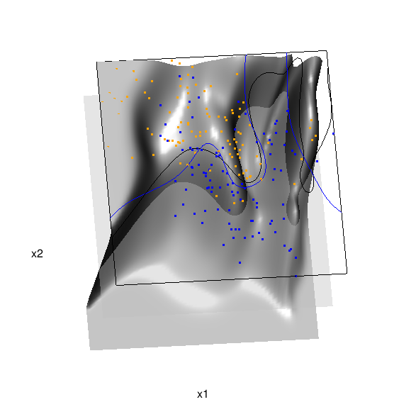
In the above graphic, the solid blue line represents the true Bayes decision boundary (i.e., {x: Pr("orange"|x) = 0.5}), which is computed from the model used to simulate these data. The probability surface (generated by the local logistic regression) is represented in gray, and the corresponding Bayes decision boundary occurs where the plane f(x) = 0.5 (in light gray) intersects with the probability surface. The solid black line is a projection of this intersection. Here is a link to the interactive version of this graphic: local logistic regression.

Below is the code and graphic associated with the kernel density classification (note: this code below should only be executed after the above code, since the 3D graphic is modified, rather than created anew):

## clear the surface, decision plane, and decision boundary
pop3d(id=sfc); pop3d(id=qds)
for(pl in pls) pop3d(id=pl)
 
## kernel density classification
## compute kernel density estimates for each class
dens.kde <-
  lapply(unique(ddat$y), function(uy) {
    apply(dat$xnew, 1, function(x0) {
      ## subset to current class
      dsub <- subset(ddat, y==uy)
      ## smoothing parameter
      l <- 1/2
      ## kernel density estimate at x0
      mean(dnorm(dsub$x1-x0[1], 0, l)*dnorm(dsub$x2-x0[2], 0, l))
    })
  })
 
## compute prior for each class (sample proportion)
prir.kde <- table(ddat$y)/length(dat$y)
 
## compute posterior probability Pr(y=1|x)
probs.kde <- prir.kde[2]*dens.kde[[2]]/
  (prir.kde[1]*dens.kde[[1]]+prir.kde[2]*dens.kde[[2]])
 
## plot classification boundary associated
## with kernel density classification
dat$probm.kde <- with(dat, matrix(probs.kde, length(px1), length(px2)))
dat$cls.kde <- with(dat, contourLines(px1, px2, probm.kde, levels=0.5))
pls <- lapply(dat$cls.kde, function(p) lines3d(p$x, p$y, z=1))
 
## plot probability surface and decision plane
sfc <- surface3d(dat$px1, dat$px2, probs.kde, alpha=1.0,
                 color="gray", specular="gray")
qds <- quads3d(x1r[c(1,2,2,1)], x2r[c(1,1,2,2)], 0.5, alpha=0.4,
               color="gray", lit=FALSE)

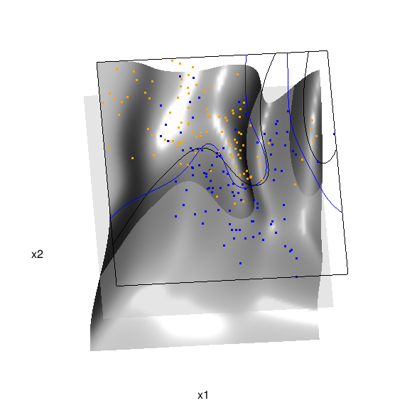
Here are links to the interactive versions of both graphics: local logistic regression, kernel density classification

This entry was posted in Technical and tagged data, graphics, programming, R, statistics on February 7, 2015.

转自：http://biostatmatt.com/archives/2678