Understanding Variational Autoencoders (VAEs)
Understanding Variational Autoencoders (VAEs)
2019-09-29 11:33:18
This blog is from: https://towardsdatascience.com/understanding-variational-autoencoders-vaes-f70510919f73
Introduction
In the last few years, deep learning based generative models have gained more and more interest due to (and implying) some amazing improvements in the field. Relying on huge amount of data, well-designed networks architectures and smart training techniques, deep generative models have shown an incredible ability to produce highly realistic pieces of content of various kind, such as images, texts and sounds. Among these deep generative models, two major families stand out and deserve a special attention: Generative Adversarial Networks (GANs) and Variational Autoencoders (VAEs).

Face images generated with a Variational Autoencoder (source: Wojciech Mormul on Github).
In a previous post, published in January of this year, we discussed in depth Generative Adversarial Networks (GANs) and showed, in particular, how adversarial training can oppose two networks, a generator and a discriminator, to push both of them to improve iteration after iteration. We introduce now, in this post, the other major kind of deep generative models: Variational Autoencoders (VAEs). In a nutshell, a VAE is an autoencoder whose encodings distribution is regularised during the training in order to ensure that its latent space has good properties allowing us to generate some new data. Moreover, the term “variational” comes from the close relation there is between the regularisation and the variational inference method in statistics.
If the last two sentences summarise pretty well the notion of VAEs, they can also raise a lot of questions. What is an autoencoder? What is the latent space and why regularising it? How to generate new data from VAEs? What is the link between VAEs and variational inference? In order to describe VAEs as well as possible, we will try to answer all this questions (and many others!) and to provide the reader with as much insights as we can (ranging from basic intuitions to more advanced mathematical details). Thus, the purpose of this post is not only to discuss the fundamental notions Variational Autoencoders rely on but also to build step by step and starting from the very beginning the reasoning that leads to these notions.
Without further ado, let’s (re)discover VAEs together!
Outline
In the first section, we will review some important notions about dimensionality reduction and autoencoder that will be useful for the understanding of VAEs. Then, in the second section, we will show why autoencoders cannot be used to generate new data and will introduce Variational Autoencoders that are regularised versions of autoencoders making the generative process possible. Finally in the last section we will give a more mathematical presentation of VAEs, based on variational inference.
Note. In the last section we have tried to make the mathematical derivation as complete and clear as possible to bridge the gap between intuitions and equations. However, the readers that doesn’t want to dive into the mathematical details of VAEs can skip this section without hurting the understanding of the main concepts. Notice also that in this post we will make the following abuse of notation: for a random variable z, we will denote p(z) the distribution (or the density, depending on the context) of this random variable.
Dimensionality reduction, PCA and autoencoders
In this first section we will start by discussing some notions related to dimensionality reduction. In particular, we will review briefly principal component analysis (PCA) and autoencoders, showing how both ideas are related to each others.
What is dimensionality reduction?
In machine learning, dimensionality reduction is the process of reducing the number of features that describe some data. This reduction is done either by selection (only some existing features are conserved) or by extraction (a reduced number of new features are created based on the old features) and can be useful in many situations that require low dimensional data (data visualisation, data storage, heavy computation…). Although there exists many different methods of dimensionality reduction, we can set a global framework that is matched by most (if not any!) of these methods.
First, let’s call encoder the process that produce the “new features” representation from the “old features” representation (by selection or by extraction) and decoder the reverse process. Dimensionality reduction can then be interpreted as data compression where the encoder compress the data (from the initial space to the encoded space, also called latent space) whereas the decoder decompress them. Of course, depending on the initial data distribution, the latent space dimension and the encoder definition, this compression can be lossy, meaning that a part of the information is lost during the encoding process and cannot be recovered when decoding.
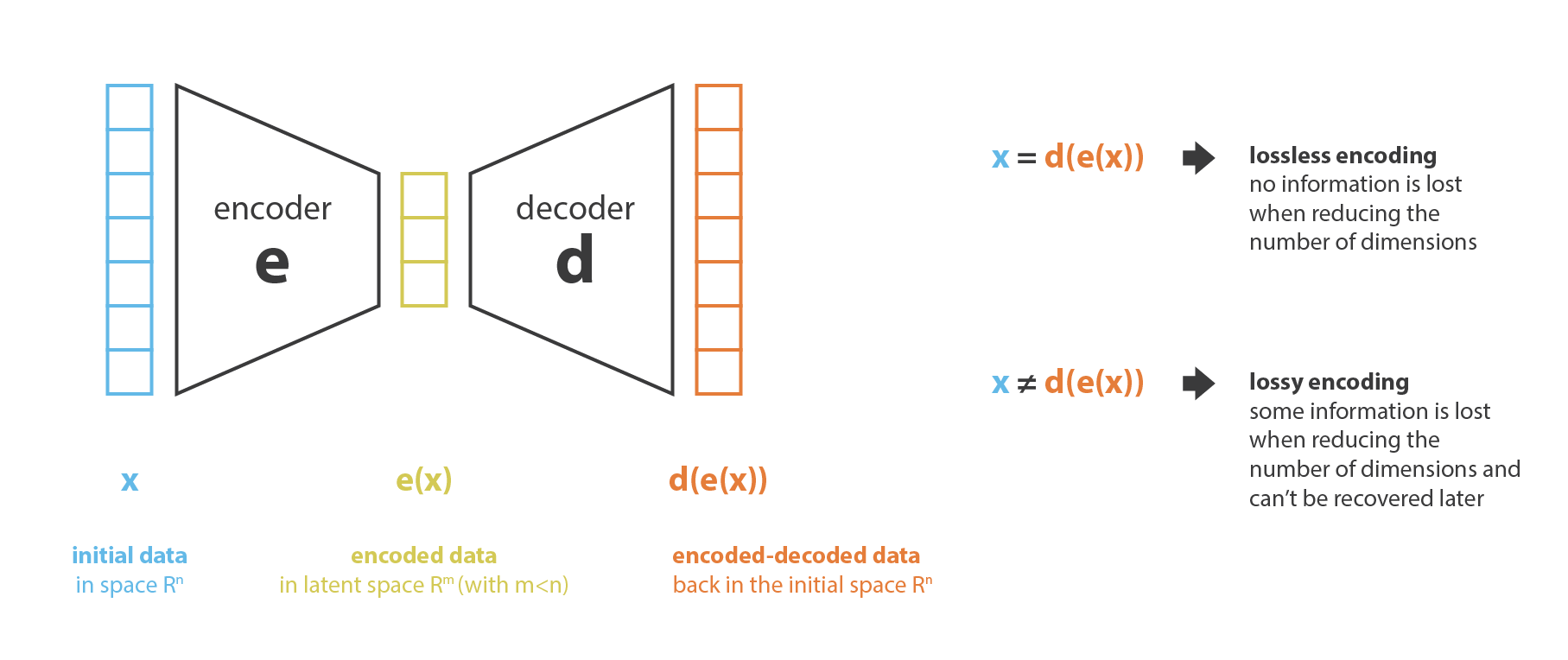
Illustration of the dimensionality reduction principle with encoder and decoder.
The main purpose of a dimensionality reduction method is to find the best encoder/decoder pair among a given family. In other words, for a given set of possible encoders and decoders, we are looking for the pair that keeps the maximum of information when encoding and, so, has the minimum of reconstruction error when decoding. If we denote respectively E and D the families of encoders and decoders we are considering, then the dimensionality reduction problem can be written

where

defines the reconstruction error measure between the input data x and the encoded-decoded data d(e(x)). Notice finally that in the following we will denote N the number of data, n_d the dimension of the initial (decoded) space and n_e the dimension of the reduced (encoded) space.
Principal components analysis (PCA)
One of the first methods that come in mind when speaking about dimensionality reduction is principal component analysis (PCA). In order to show how it fits the framework we just described and make the link towards autoencoders, let’s give a very high overview of how PCA works, letting most of the details aside (notice that we plan to write a full post on the subject).
The idea of PCA is to build n_e new independent features that are linear combinations of the n_d old features and so that the projections of the data on the subspace defined by these new features are as close as possible to the initial data (in term of euclidean distance). In other words, PCA is looking for the best linear subspace of the initial space (described by an orthogonal basis of new features) such that the error of approximating the data by their projections on this subspace is as small as possible.
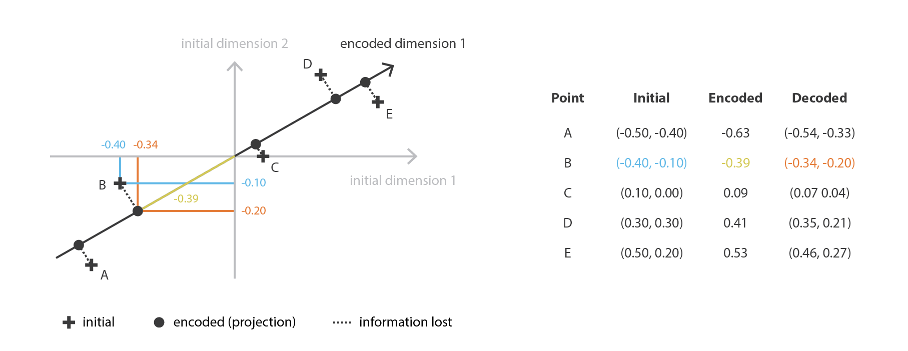
Principal Component Analysis (PCA) is looking for the best linear subspace using linear algebra.
Translated in our global framework, we are looking for an encoder in the family E of the n_e by n_d matrices (linear transformation) whose rows are orthonormal (features independence) and for the associated decoder among the family D of n_d by n_e matrices. It can be shown that the unitary eigenvectors corresponding to the n_e greatest eigenvalues (in norm) of the covariance features matrix are orthogonal (or can be chosen to be so) and define the best subspace of dimension n_e to project data on with minimal error of approximation. Thus, these n_e eigenvectors can be chosen as our new features and, so, the problem of dimension reduction can then be expressed as an eigenvalue/eigenvector problem. Moreover, it can also be shown that, in such case, the decoder matrix is the transposed of the encoder matrix.
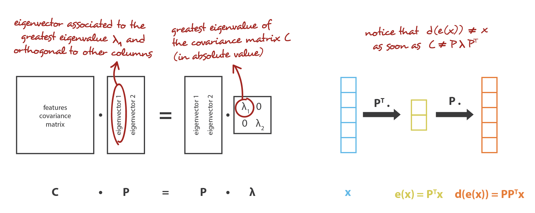
PCA matches the encoder-decoder framework we described.
Autoencoders
Let’s now discuss autoencoders and see how we can use neural networks for dimensionality reduction. The general idea of autoencoders is pretty simple and consists in setting an encoder and a decoder as neural networks and to learn the best encoding-decoding scheme using an iterative optimisation process. So, at each iteration we feed the autoencoder architecture (the encoder followed by the decoder) with some data, we compare the encoded-decoded output with the initial data and backpropagate the error through the architecture to update the weights of the networks.
Thus, intuitively, the overall autoencoder architecture (encoder+decoder) creates a bottleneck for data that ensures only the main structured part of the information can go through and be reconstructed. Looking at our general framework, the family E of considered encoders is defined by the encoder network architecture, the family D of considered decoders is defined by the decoder network architecture and the search of encoder and decoder that minimise the reconstruction error is done by gradient descent over the parameters of these networks.

Illustration of an autoencoder with its loss function.
Let’s first suppose that both our encoder and decoder architectures have only one layer without non-linearity (linear autoencoder). Such encoder and decoder are then simple linear transformations that can be expressed as matrices. In such situation, we can see a clear link with PCA in the sense that, just like PCA does, we are looking for the best linear subspace to project data on with as few information loss as possible when doing so. Encoding and decoding matrices obtained with PCA define naturally one of the solutions we would be satisfied to reach by gradient descent, but we should outline that this is not the only one. Indeed, several basis can be chosen to describe the same optimal subspace and, so, several encoder/decoder pairs can give the optimal reconstruction error. Moreover, for linear autoencoders and contrarily to PCA, the new features we end up do not have to be independent (no orthogonality constraints in the neural networks).
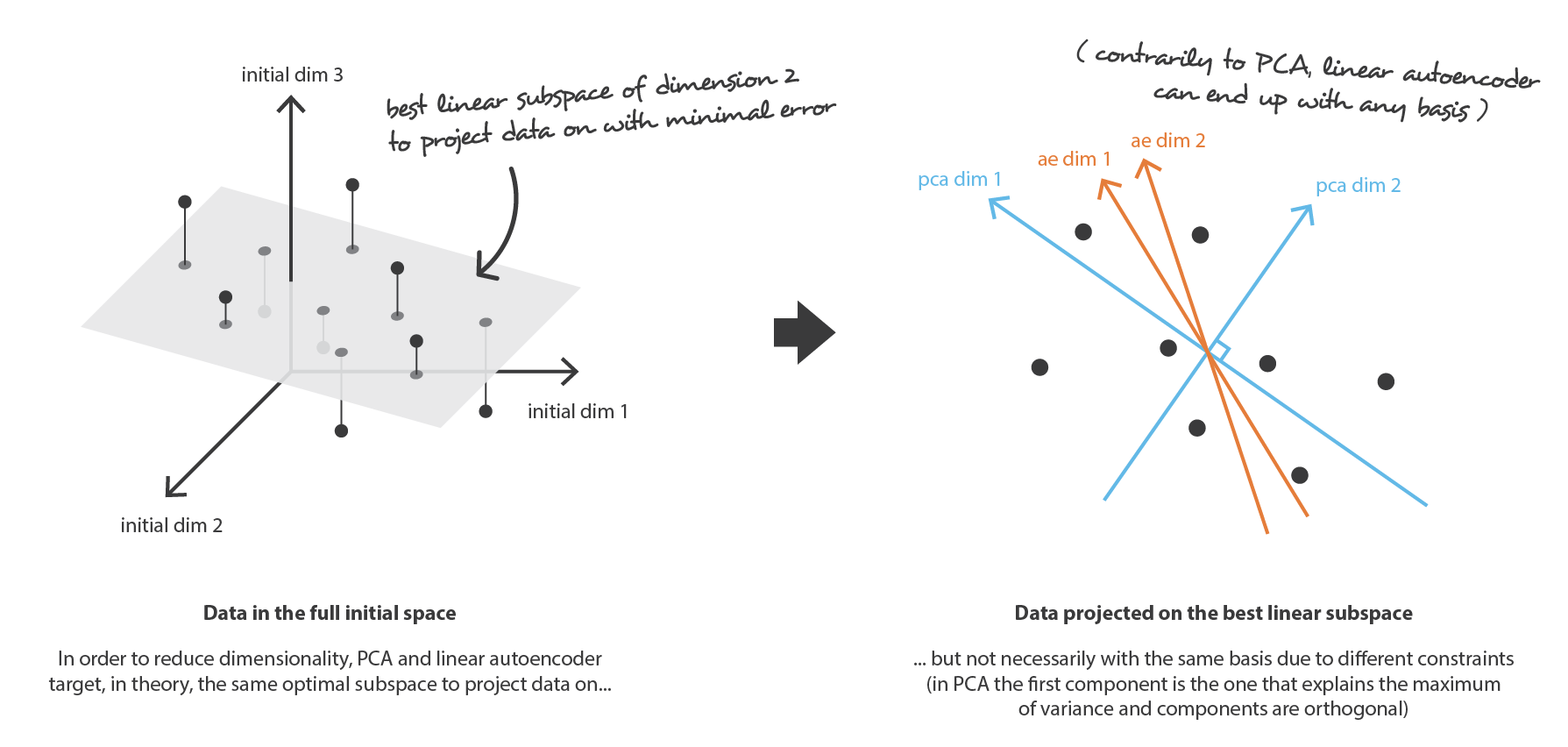
Link between linear autoencoder and PCA.
Now, let’s assume that both the encoder and the decoder are deep and non-linear. In such case, the more complex the architecture is, the more the autoencoder can proceed to a high dimensionality reduction while keeping reconstruction loss low. Intuitively, if our encoder and our decoder have enough degrees of freedom, we can reduce any initial dimensionality to 1. Indeed, an encoder with “infinite power” could theoretically takes our N initial data points and encodes them as 1, 2, 3, … up to N (or more generally, as N integer on the real axis) and the associated decoder could make the reverse transformation, with no loss during the process.
Here, we should however keep two things in mind. First, an important dimensionality reduction with no reconstruction loss often comes with a price: the lack of interpretable and exploitable structures in the latent space (lack of regularity). Second, most of the time the final purpose of dimensionality reduction is not to only reduce the number of dimensions of the data but to reduce this number of dimensions while keeping the major part of the data structure information in the reduced representations. For these two reasons, the dimension of the latent space and the “depth” of autoencoders (that define degree and quality of compression) have to be carefully controlled and adjusted depending on the final purpose of the dimensionality reduction.
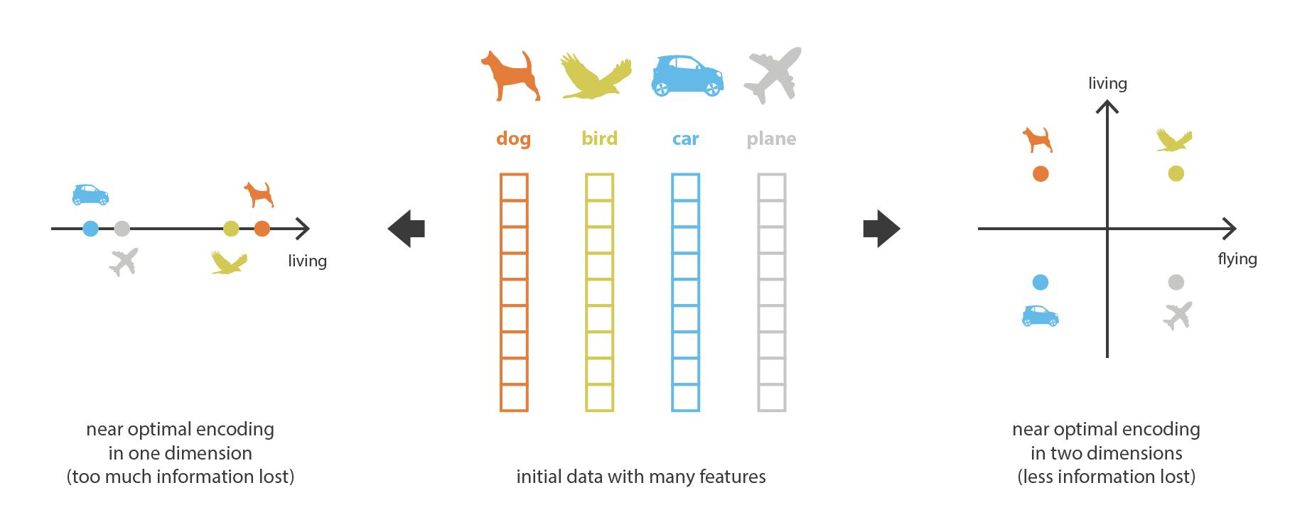
When reducing dimensionality, we want to keep the main structure there exists among the data.
Variational Autoencoders
Up to now, we have discussed dimensionality reduction problem and introduce autoencoders that are encoder-decoder architectures that can be trained by gradient descent. Let’s now make the link with the content generation problem, see the limitations of autoencoders in their current form for this problem and introduce Variational Autoencoders.
Limitations of autoencoders for content generation
At this point, a natural question that comes in mind is “what is the link between autoencoders and content generation?”. Indeed, once the autoencoder has been trained, we have both an encoder and a decoder but still no real way to produce any new content. At first sight, we could be tempted to think that, if the latent space is regular enough (well “organized” by the encoder during the training process), we could take a point randomly from that latent space and decode it to get a new content. The decoder would then act more or less like the generator of a Generative Adversarial Network.
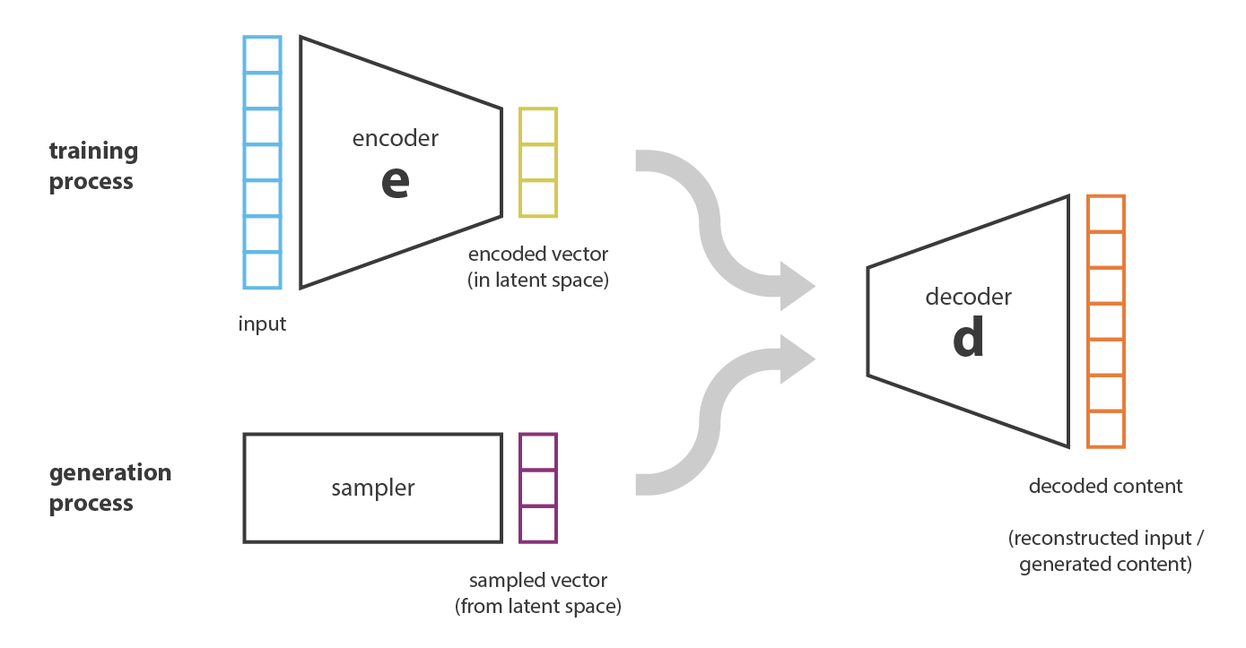
We can generate new data by decoding points that are randomly sampled from the latent space. The quality and relevance of generated data depend on the regularity of the latent space.
However, as we discussed in the previous section, the regularity of the latent space for autoencoders is a difficult point that depends on the distribution of the data in the initial space, the dimension of the latent space and the architecture of the encoder. So, it is pretty difficult (if not impossible) to ensure, a priori, that the encoder will organize the latent space in a smart way compatible with the generative process we just described.
To illustrate this point, let’s consider the example we gave previously in which we described an encoder and a decoder powerful enough to put any N initial training data onto the real axis (each data point being encoded as a real value) and decode them without any reconstruction loss. In such case, the high degree of freedom of the autoencoder that makes possible to encode and decode with no information loss (despite the low dimensionality of the latent space) leads to a severe overfitting implying that some points of the latent space will give meaningless content once decoded. If this one dimensional example has been voluntarily chosen to be quite extreme, we can notice that the problem of the autoencoders latent space regularity is much more general than that and deserve a special attention.

Irregular latent space prevent us from using autoencoder for new content generation.
When thinking about it for a minute, this lack of structure among the encoded data into the latent space is pretty normal. Indeed, nothing in the task the autoencoder is trained for enforce to get such organisation: the autoencoder is solely trained to encode and decode with as few loss as possible, no matter how the latent space is organised. Thus, if we are not careful about the definition of the architecture, it is natural that, during the training, the network takes advantage of any overfitting possibilities to achieve its task as well as it can… unless we explicitly regularise it!
Definition of variational autoencoders
So, in order to be able to use the decoder of our autoencoder for generative purpose, we have to be sure that the latent space is regular enough. One possible solution to obtain such regularity is to introduce explicit regularisation during the training process. Thus, as we briefly mentioned in the introduction of this post, a variational autoencoder can be defined as being an autoencoder whose training is regularised to avoid overfitting and ensure that the latent space has good properties that enable generative process.
Just as a standard autoencoder, a variational autoencoder is an architecture composed of both an encoder and a decoder and that is trained to minimise the reconstruction error between the encoded-decoded data and the initial data. However, in order to introduce some regularisation of the latent space, we proceed to a slight modification of the encoding-decoding process: instead of encoding an input as a single point, we encode it as a distribution over the latent space. The model is then trained as follows:
- first, the input is encoded as distribution over the latent space
- second, a point from the latent space is sampled from that distribution
- third, the sampled point is decoded and the reconstruction error can be computed
- finally, the reconstruction error is backpropagated through the network

Difference between autoencoder (deterministic) and variational autoencoder (probabilistic).
In practice, the encoded distributions are chosen to be normal so that the encoder can be trained to return the mean and the covariance matrix that describe these Gaussians. The reason why an input is encoded as a distribution with some variance instead of a single point is that it makes possible to express very naturally the latent space regularisation: the distributions returned by the encoder are enforced to be close to a standard normal distribution. We will see in the next subsection that we ensure this way both a local and global regularisation of the latent space (local because of the variance control and global because of the mean control).
Thus, the loss function that is minimised when training a VAE is composed of a “reconstruction term” (on the final layer), that tends to make the encoding-decoding scheme as performant as possible, and a “regularisation term” (on the latent layer), that tends to regularise the organisation of the latent space by making the distributions returned by the encoder close to a standard normal distribution. That regularisation term is expressed as the Kulback-Leibler divergence between the returned distribution and a standard Gaussian and will be further justified in the next section. We can notice that the Kullback-Leibler divergence between two Gaussian distributions has a closed form that can be directly expressed in terms of the means and the covariance matrices of the the two distributions.

In variational autoencoders, the loss function is composed of a reconstruction term (that makes the encoding-decoding scheme efficient) and a regularisation term (that makes the latent space regular).
Intuitions about the regularisation
The regularity that is expected from the latent space in order to make generative process possible can be expressed through two main properties: continuity (two close points in the latent space should not give two completely different contents once decoded) and completeness (for a chosen distribution, a point sampled from the latent space should give “meaningful” content once decoded).
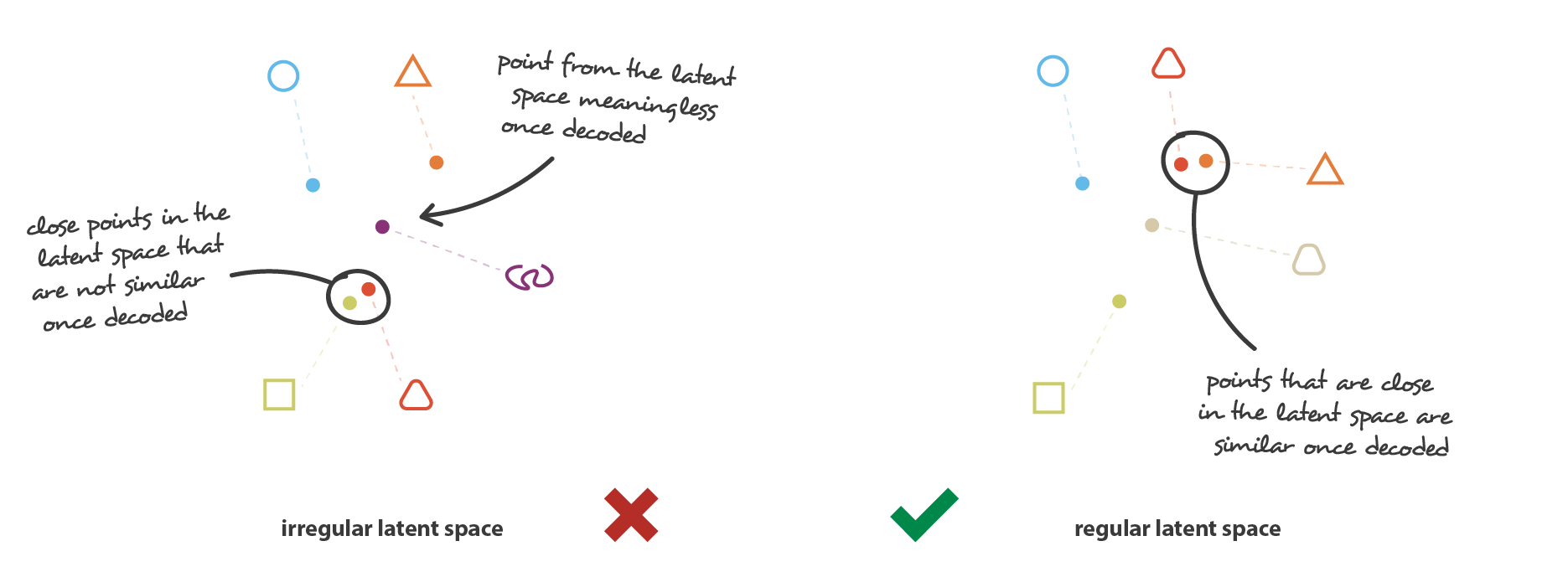
Difference between a “regular” and an “irregular” latent space.
The only fact that VAEs encode inputs as distributions instead of simple points is not sufficient to ensure continuity and completeness. Without a well defined regularisation term, the model can learn, in order to minimise its reconstruction error, to “ignore” the fact that distributions are returned and behave almost like classic autoencoders (leading to overfitting). To do so, the encoder can either return distributions with tiny variances (that would tend to be punctual distributions) or return distributions with very different means (that would then be really far apart from each other in the latent space). In both cases, distributions are used the wrong way (cancelling the expected benefit) and continuity and/or completeness are not satisfied.
So, in order to avoid these effects we have to regularise both the covariance matrix and the mean of the distributions returned by the encoder. In practice, this regularisation is done by enforcing distributions to be close to a standard normal distribution (centred and reduced). This way, we require the covariance matrices to be close to the identity, preventing punctual distributions, and the mean to be close to 0, preventing encoded distributions to be too far apart from each others.
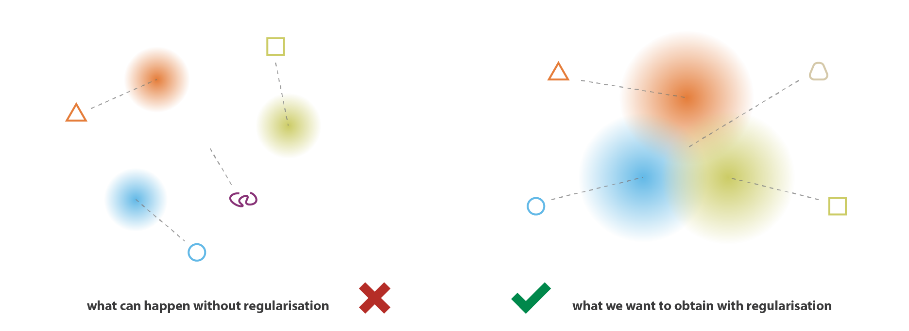
The returned distributions of VAEs have to be regularised to obtain a latent space with good properties.
With this regularisation term, we prevent the model to encode data far apart in the latent space and encourage as much as possible returned distributions to “overlap”, satisfying this way the expected continuity and completeness conditions. Naturally, as for any regularisation term, this comes at the price of a higher reconstruction error on the training data. The tradeoff between the reconstruction error and the KL divergence can however be adjusted and we will see in the next section how the expression of the balance naturally emerge from our formal derivation.
To conclude this subsection, we can observe that continuity and completeness obtained with regularisation tend to create a “gradient” over the information encoded in the latent space. For example, a point of the latent space that would be halfway between the means of two encoded distributions coming from different training data should be decoded in something that is somewhere between the data that gave the first distribution and the data that gave the second distribution as it may be sampled by the autoencoder in both cases.
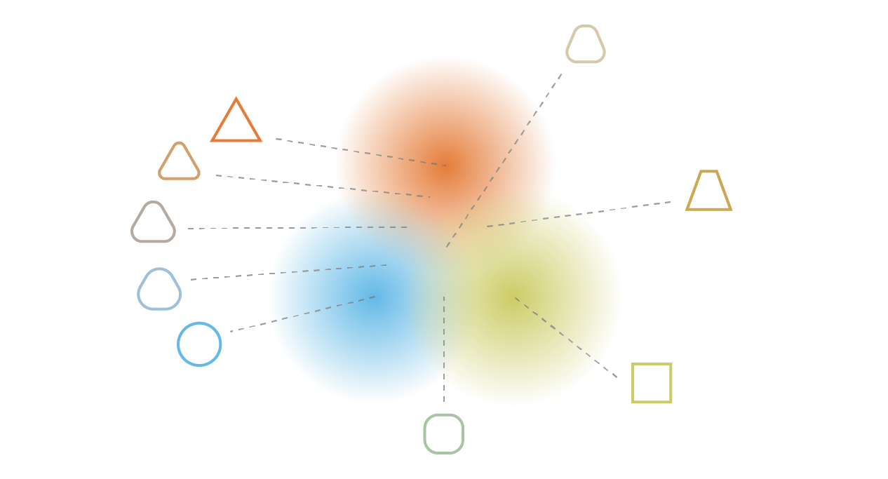
Regularisation tends to create a “gradient” over the information encoded in the latent space.
Note. As a side note, we can mention that the second potential problem we have mentioned (the network put distributions far from each others) is in fact almost equivalent to the first one (the network tends to return punctual distribution) up to a change of scale: in both case variances of distributions become small relatively to distance between their means.
Mathematical details of VAEs
In the previous section we gave the following intuitive overview: VAEs are autoencoders that encode inputs as distributions instead of points and whose latent space “organisation” is regularised by constraining distributions returned by the encoder to be close to a standard Gaussian. In this section we will give a more mathematical view of VAEs that will allow us to justify the regularisation term more rigorously. To do so, we will set a clear probabilistic framework and will use, in particular, variational inference technique.
Probabilistic framework and assumptions
Let’s begin by defining a probabilistic graphical model to describe our data. We denote by x the variable that represents our data and assume that x is generated from a latent variable z (the encoded representation) that is not directly observed. Thus, for each data point, the following two steps generative process is assumed:
- first, a latent representation z is sampled from the prior distribution p(z)
- second, the data x is sampled from the conditional likelihood distribution p(x|z)
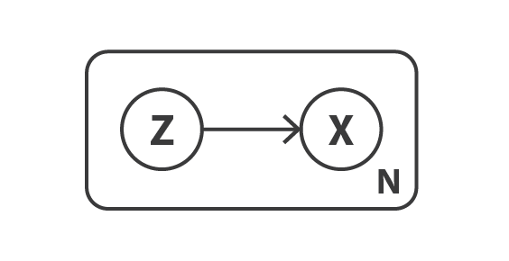
Graphical model of the data generation process.
With such a probabilistic model in mind, we can redefine our notions of encoder and decoder. Indeed, contrarily to a simple autoencoder that consider deterministic encoder and decoder, we are going to consider now probabilistic versions of these two objects. The “probabilistic decoder” is naturally defined by p(x|z), that describes the distribution of the decoded variable given the encoded one, whereas the “probabilistic encoder” is defined by p(z|x), that describes the distribution of the encoded variable given the decoded one.
At this point, we can already notice that the regularisation of the latent space that we lacked in simple autoencoders naturally appears here in the definition of the data generation process: encoded representations z in the latent space are indeed assumed to follow the prior distribution p(z). Otherwise, we can also remind the the well-known Bayes theorem that makes the link between the prior p(z), the likelihood p(x|z), and the posterior p(z|x)

Let’s now make the assumption that p(z) is a standard Gaussian distribution and that p(x|z) is a Gaussian distribution whose mean is defined by a deterministic function f of the variable of z and whose covariance matrix has the form of a positive constant c that multiplies the identity matrix I. The function f is assumed to belong to a family of functions denoted F that is left unspecified for the moment and that will be chosen later. Thus, we have

Let’s consider, for now, that f is well defined and fixed. In theory, as we know p(z) and p(x|z), we can use the Bayes theorem to compute p(z|x): this is a classical Bayesian inference problem. However, as we discussed in our previous article, this kind of computation is often intractable (because of the integral at the denominator) and require the use of approximation techniques such as variational inference.
Note. Here we can mention that p(z) and p(x|z) are both Gaussian distributions, implying that p(z|x) should also follow a Gaussian distribution. In theory, we could then “only” try to express the mean and the covariance matrix of p(z|x) with respect to the means and the covariance matrices of p(z) and p(x|z). However, in practice these values depend on the function f that can be complex and that is not defined for now (even if we have assumed the contrary). Moreover, the use of an approximation technique like variational inference makes the approach pretty general and more robust to some changes in the hypothesis of the model.
Variational inference formulation
In statistics, variational inference (VI) is a technique to approximate complex distributions. The idea is to set a parametrised family of distribution (for example the family of Gaussians, whose parameters are the mean and the covariance) and to look for the best approximation of our target distribution among this family. The best element in the family is one that minimise a given approximation error measurement (most of the time the Kullback-Leibler divergence between approximation and target) and is found by gradient descent over the parameters that describe the family. For more details, we refer to our post on variational inference and references therein.
Here we are going to approximate p(z|x) by a Gaussian distribution q_x(z) whose mean and covariance are defined by two functions, g and h, of the parameter x. These two functions are supposed to belong, respectively, to the families of functions G and H that will be specified later but that are supposed to be parametrised. Thus we can denote

So, we have defined this way a family of candidates for variational inference and need now to find the best approximation among this family by optimising the functions g and h (in fact, their parameters) to minimise the Kullback-Leibler divergence between the approximation and the target p(z|x). In other words, we are looking for the optimal g* and h* such that

In the second last equation, we can observe the tradeoff there exists — when approximating the posterior p(z|x) — between maximising the likelihood of the “observations” (maximisation of the expected log-likelihood, for the first term) and staying close to the prior distribution (minimisation of the KL divergence between q_x(z) and p(z), for the second term). This tradeoff is natural for Bayesian inference problem and express the balance that needs to be found between the confidence we have in the data and the confidence we have in the prior.
Up to know, we have assumed the function f known and fixed and we have showed that, under such assumptions, we can approximate the posterior p(z|x) using variational inference technique. However, in practice this function f, that defines the decoder, is not known and also need to be chosen. To do so, let’s remind that our initial goal is to find a performant encoding-decoding scheme whose latent space is regular enough to be used for generative purpose. If the regularity is mostly ruled by the prior distribution assumed over the latent space, the performance of the overall encoding-decoding scheme highly depends on the choice of the function f. Indeed, as p(z|x) can be approximate (by variational inference) from p(z) and p(x|z) and as p(z) is a simple standard Gaussian, the only two levers we have at our disposal in our model to make optimisations are the parameter c (that defines the variance of the posterior) and the function f (that defines the mean of the posterior).
So, let’s consider that, as we discussed earlier, we can get for any function f in F (each defining a different probabilistic decoder p(x|z)) the best approximation of p(z|x), denoted q*_x(z). Despite its probabilistic nature, we are looking for an encoding-decoding scheme as efficient as possible and, then, we want to choose the function f that maximises the expected log-likelihood of x given z when z is sampled from q*_x(z). In other words, for a given input x, we want to maximise the probability to have x̂ = x when we sample z from the distribution q*_x(z) and then sample x̂ from the distribution p(x|z). Thus, we are looking for the optimal f* such that

where q*_x(z) depends on the function f and is obtained as described before. Gathering all the pieces together, we are looking for optimal f*, g* and h* such that

We can identify in this objective function the elements introduced in the intuitive description of VAEs given in the previous section: the reconstruction error between x and f(z) and the regularisation term given by the KL divergence between q_x(z) and p(z) (which is a standard Gaussian). We can also notice the constant c that rules the balance between the two previous terms. The higher c is the more we assume a high variance around f(z) for the probabilistic decoder in our model and, so, the more we favour the regularisation term over the reconstruction term (and the opposite stands if c is low).
Bringing neural networks into the model
Up to know, we have set a probabilistic model that depends on three functions, f, g and h, and express, using variational inference, the optimisation problem to solve in order to get f*, g* and h* that give the optimal encoding-decoding scheme with this model. As we can’t easily optimise over the entire space of functions, we constrain the optimisation domain and decide to express f, g and h as neural networks. Thus, F, G and H correspond respectively to the families of functions defined by the networks architectures and the optimisation is done over the parameters of these networks.
In practice, g and h are not defined by two completely independent networks but share a part of their architecture and their weights so that we have

As it defines the covariance matrix of q_x(z), h(x) is supposed to be a square matrix. However, in order to simplify the computation and reduce the number of parameters, we make the additional assumption that our approximation of p(z|x), q_x(z), is a multidimensional Gaussian distribution with diagonal covariance matrix (variables independence assumption). With this assumption, h(x) is simply the vector of the diagonal elements of the covariance matrix and has then the same size as g(x). However, we reduce this way the family of distributions we consider for variational inference and, so, the approximation of p(z|x) obtained can be less accurate.
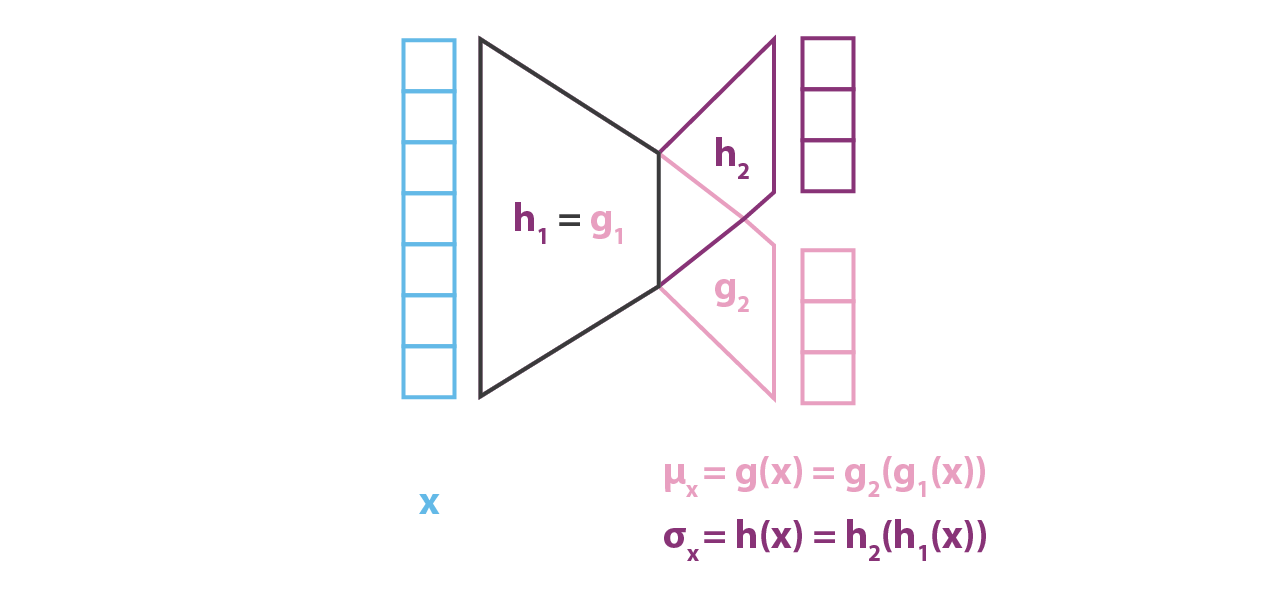
Encoder part of the VAE.
Contrarily to the encoder part that models p(z|x) and for which we considered a Gaussian with both mean and covariance that are functions of x (g and h), our model assumes for p(x|z) a Gaussian with fixed covariance. The function f of the variable z defining the mean of that Gaussian is modelled by a neural network and can be represented as follows

Decoder part of the VAE.
The overall architecture is then obtained by concatenating the encoder and the decoder parts. However we still need to be very careful about the way we sample from the distribution returned by the encoder during the training. The sampling process has to be expressed in a way that allows the error to be backpropagated through the network. A simple trick, called reparametrisation trick, is used to make the gradient descent possible despite the random sampling that occurs halfway of the architecture and consists in using the fact that if z is a random variable following a Gaussian distribution with mean g(x) and with covariance h(x) then it can be expressed as

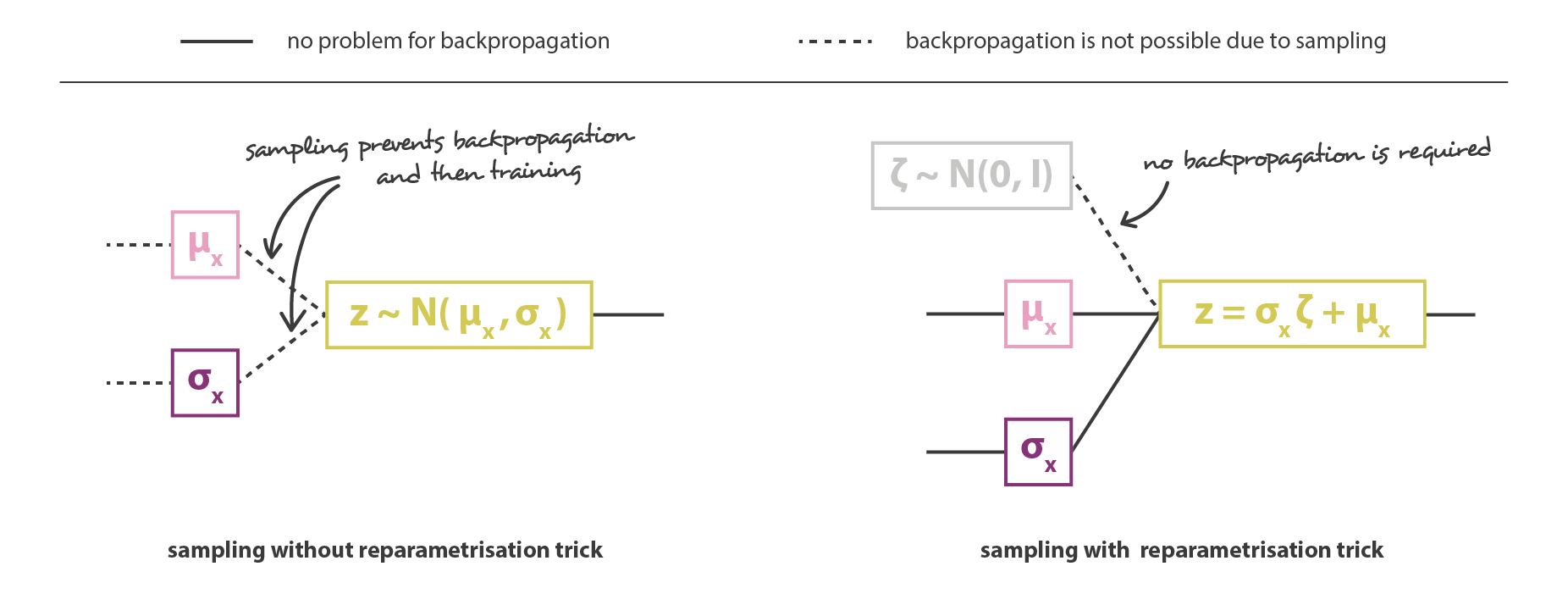
Illustration of the reparametrisation trick.
Finally, the objective function of the variational autoencoder architecture obtained this way is given by the last equation of the previous subsection in which the theoretical expectancy is replaced by a more or less accurate Monte-Carlo approximation that consists, most of the time, into a single draw. So, considering this approximation and denoting C = 1/(2c), we recover the loss function derived intuitively in the previous section, composed of a reconstruction term, a regularisation term and a constant to define the relative weights of these two terms.

Variational Autoencoders representation.
Takeaways
The main takeways of this article are:
- dimensionality reduction is the process of reducing the number of features that describe some data (either by selecting only a subset of the initial features or by combining them into a reduced number new features) and, so, can be seen as an encoding process
- autoencoders are neural networks architectures composed of both an encoder and a decoder that create a bottleneck to go through for data and that are trained to lose a minimal quantity of information during the encoding-decoding process (training by gradient descent iterations with the goal to reduce the reconstruction error)
- due to overfitting, the latent space of an autoencoder can be extremely irregular (close points in latent space can give very different decoded data, some point of the latent space can give meaningless content once decoded, …) and, so, we can’t really define a generative process that simply consists to sample a point from the latent space and make it go through the decoder to get a new data
- variational autoencoders (VAEs) are autoencoders that tackle the problem of the latent space irregularity by making the encoder return a distribution over the latent space instead of a single point and by adding in the loss function a regularisation term over that returned distribution in order to ensure a better organisation of the latent space
- assuming a simple underlying probabilistic model to describe our data, the pretty intuitive loss function of VAEs, composed of a reconstruction term and a regularisation term, can be carefully derived, using in particular the statistical technique of variational inference (hence the name “variational” autoencoders)
To conclude, we can outline that, during the last years, GANs have benefited from much more scientific contributions than VAEs. Among other reasons, the higher interest that has been shown by the community for GANs can be partly explained by the higher degree of complexity in VAEs theoretical basis (probabilistic model and variational inference) compared to the simplicity of the adversarial training concept that rules GANs. With this post we hope that we managed to share valuable intuitions as well as strong theoretical foundations to make VAEs more accessible to newcomers, as we did for GANs earlier this year. However, now that we have discussed in depth both of them, one question remains… are you more GANs or VAEs?
Thanks for reading!
Understanding Variational Autoencoders (VAEs)的更多相关文章
- (译) Conditional Variational Autoencoders 条件式变换自编码机
Conditional Variational Autoencoders --- 条件式变换自编码机 Goal of a Variational Autoencoder: 一个 VAE(variati ...
- 条件式变分自编码机(Conditional Variational Autoencoders)
Conditional Variational Autoencoders 条件式变换自编码机 摘要: Conditional Variational Autoencoders --- 条件式变换自编码 ...
- [Bayesian] “我是bayesian我怕谁”系列 - Variational Autoencoders
本是neural network的内容,但偏偏有个variational打头,那就聊聊.涉及的内容可能比较杂,但终归会 end with VAE. 各个概念的详细解释请点击推荐的链接,本文只是重在理清 ...
- 基于图嵌入的高斯混合变分自编码器的深度聚类(Deep Clustering by Gaussian Mixture Variational Autoencoders with Graph Embedding, DGG)
基于图嵌入的高斯混合变分自编码器的深度聚类 Deep Clustering by Gaussian Mixture Variational Autoencoders with Graph Embedd ...
- Variational Autoencoders and Nonlinear ICA: A Unifying Framework
目录 概 主要内容 本文的模型 Identifiability Khemakhem I., Kingma D. P., Monti R. P. and Hyv"{a}rinen A. Var ...
- Improving Variational Auto-Encoders using Householder Flow
目录 概 主要内容 代码 Tomczak J. and Welling M. Improving Variational Auto-Encoders using Householder Flow. N ...
- Variational Auto-Encoders原理
目录 AE v.s. VAE Generative model VAE v.s. GAN AE v.s. VAE Generative model VAE v.s. GAN
- PP: Time series anomaly detection with variational autoencoders
Problem: unsupervised anomaly detection Model: VAE-reEncoder VAE with two encoders and one decoder. ...
- [2018 ACL Long] 对话系统
[NLG - E2E - knowledge guide generation] 1. Knowledge Diffusion for Neural Dialogue Generation ( Ci ...
随机推荐
- Android源码分析(七)-----如何解决java编译版本问题
一 : 问题描述 Your version is: java version "1.6.0_31" Java(TM) SE Runtime Environment (build 1 ...
- Vue 中 $nextTick() 的应用
Vue 在更新 DOM 时是异步执行的. 只要侦听到数据变化,Vue 将开启一个队列,并缓冲在同一事件循环中发生的所有数据变更.如果同一个 watcher 被多次触发,只会被推入到队列中一次.这种在缓 ...
- jmeter使用小结
写这篇短文主要想详细介绍一下jmeter中取样器.逻辑控制器.前置处理器.后置处理器.定时器.配置元件等,可能看起来比较繁杂,其实里面很多操作是类似的,一篇总结和记录的博客: jmeter官方用户手册 ...
- php根据二维数组中的某一元素相等,另一个元素相加
二维数组:$taskData Array ( [0] => Array ( [area] => 1 [winsFlag] => 7 [count] => 3 ) [1] =&g ...
- 自己开发SSO单点登录
概述 单点登录指的是有一个中央的单点登录服务器,各个子系统和这个中央的单点登录服务器打交道,比如有A,B两个子系统. A登录后,B系统就不用再登录,直接可以访问,当其中有一个子系统选择注销时,那么所有 ...
- Odoo中的self详解
转载请注明原文地址:https://www.cnblogs.com/ygj0930/p/10826307.html 一:self是什么 目前新版的Odoo中使用到的self,是对 游标cr.用户ID ...
- 让Windows中的文件名支持大小写
背景 最近在Linux官网下载了Linux内核,下载下来的是一个后缀为.tar.xz的压缩包,于是在毫不知情的情况下随随便便解压了,解压过程中出现了很多问题. 其中一个问题就是在Windows下,不区 ...
- 使用django的MTV开发模式返回一个网页
1.MTV开发模式介绍 M:Models 模型(数据) 与数据组织相关的功能.组织和存储数据的方法和模式,与数据模型相关的操作. T:Templates 模板(样式) 与表现相关的所有功能.页面展示风 ...
- JSR303后端校验(一)
JSR303后端校验(一) (1)在pom文件中添加依赖 <!-- JSR303后端校验 --> <dependency> <groupId>org.hiberna ...
- scala中可以执行外部命令Process
后续用到在总结 Process(s"hadoop fs -rm -r ${path}").!!
