（六）6.16 Neurons Networks linear decoders and its implements

Sparse AutoEncoder是一个三层结构的网络，分别为输入输出与隐层，前边自编码器的描述可知，神经网络中的神经元都采用相同的激励函数，Linear Decoders 修改了自编码器的定义，对输出层与隐层采用了不用的激励函数，所以 Linear Decoder 得到的模型更容易应用，而且对模型的参数变化有更高的鲁棒性。

在网络中的前向传导过程中的公式：

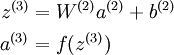
其中 a⁽³⁾ 是输出. 在自编码器中, a⁽³⁾ 近似重构了输入 x = a⁽¹⁾ 。

对于最后一层为 sigmod(tanh) 激活函数的 autoencoder ，会直接将数据归一化到 [0,1] ，所以当 f(z⁽³⁾) 采用 sigmod(tanh) 函数时，就要对输入限制或缩放，使其位于 [0,1] 范围中。但是对于输入数据 x ，比如 MNIST，但是很难满足 x 也在 [0,1] 的要求。比如， PCA 白化处理的输入并不满足 [0,1] 范围要求。

另 a⁽³⁾ = z⁽³⁾ 可以很简单的解决上述问题。即在输出端使用恒等函数 f(z) = z 作为激励函数，于是有 a⁽³⁾ = f(z⁽³⁾) = z⁽³⁾。该特殊的激励函数叫做 线性激励 (恒等激励)函数。

Linear Decoder 中隐含层的神经元依然使用 sigmod（tanh）激励函数。隐含单元的激励公式为 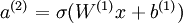 ,其中  是 S 型函数, x 是入, W⁽¹⁾ 和 b⁽¹⁾ 分别是隐单元的权重和偏差项。即仅在输出层中使用线性激励函数。这用一个 S 型或 tanh 隐含层以及线性输出层构成的自编码器，叫做线性解码器。

在线性解码器中，。因为输出  是隐单元激励输出的线性函数，改变 W⁽²⁾ ，即可使输出值 a⁽³⁾ 大于 1 或者小于 0。这样就可以避免在 sigmod 对输出层的值缩放到 [0,1] 。

随着输出单元的激励函数的改变，输出单元的梯度也相应变化。之前每一个输出单元误差项定义为：

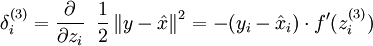
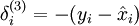
其中 y = x 是所期望的输出,  是自编码器的输出,   是激励函数.因为在输出层激励函数为 f(z) = z, 这样 f'(z) = 1，所以上述公式可以简化为

当然，若使用反向传播算法来计算隐含层的误差项时:

因为隐含层采用一个 S 型（或 tanh）的激励函数 f,在上述公式中， 依然是 S 型（或 tanh）函数的导数。即Linear Decoder中只有输出层残差是不同于autoencoder 的。

Liner Decoder 代码：

%% CS294A/CS294W Linear Decoder Exercise

%  Instructions
%  ------------
%
%  This file contains code that helps you get started on the
%  linear decoder exericse. For this exercise, you will only need to modify
%  the code in sparseAutoencoderLinearCost.m. You will not need to modify
%  any code in this file.

%%======================================================================
%% STEP 0: Initialization
%  Here we initialize some parameters used for the exercise.

imageChannels = 3;     % number of channels (rgb, so 3)

patchDim   = 8;          % patch dimension(需要 8*8 的小patches)
numPatches = 100000;   % number of patches
% 把8 * 8 * rgb_size 的小patchs 共同作为可见层的unit数目
visibleSize = patchDim * patchDim * imageChannels;  % number of input units
outputSize  = visibleSize;   % number of output units
hiddenSize  = 400;           % number of hidden units 

sparsityParam = 0.035; % desired average activation of the hidden units.
lambda = 3e-3;         % weight decay parameter
beta = 5;              % weight of sparsity penalty term       

epsilon = 0.1;	       % epsilon for ZCA whitening

%%======================================================================
%% STEP 1: Create and modify sparseAutoencoderLinearCost.m to use a linear decoder,
%          and check gradients
%  You should copy sparseAutoencoderCost.m from your earlier exercise
%  and rename it to sparseAutoencoderLinearCost.m.
%  Then you need to rename the function from sparseAutoencoderCost to
%  sparseAutoencoderLinearCost, and modify it so that the sparse autoencoder
%  uses a linear decoder instead. Once that is done, you should check
% your gradients to verify that they are correct.

% NOTE: Modify sparseAutoencoderCost first!

% To speed up gradient checking, we will use a reduced network and some
% dummy patches

debugHiddenSize = 5;
debugvisibleSize = 8;
patches = rand([8 10]);
theta = initializeParameters(debugHiddenSize, debugvisibleSize); 

[cost, grad] = sparseAutoencoderLinearCost(theta, debugvisibleSize, debugHiddenSize, ...
                                           lambda, sparsityParam, beta, ...
                                           patches);

% Check gradients
numGrad = computeNumericalGradient( @(x) sparseAutoencoderLinearCost(x, debugvisibleSize, debugHiddenSize, ...
                                                  lambda, sparsityParam, beta, ...
                                                  patches), theta);

% Use this to visually compare the gradients side by side
disp([numGrad grad]); 

diff = norm(numGrad-grad)/norm(numGrad+grad);
% Should be small. In our implementation, these values are usually less than 1e-9.
disp(diff); 

assert(diff < 1e-9, 'Difference too large. Check your gradient computation again');

% NOTE: Once your gradients check out, you should run step 0 again to
%       reinitialize the parameters
%}

%%======================================================================
%% STEP 2: Learn features on small patches
%  In this step, you will use your sparse autoencoder (which now uses a
%  linear decoder) to learn features on small patches sampled from related
%  images.

%% STEP 2a: Load patches
%  In this step, we load 100k patches sampled from the STL10 dataset and
%  visualize them. Note that these patches have been scaled to [0,1]

load stlSampledPatches.mat

displayColorNetwork(patches(:, 1:100));

%% STEP 2b: Apply preprocessing
%  In this sub-step, we preprocess the sampled patches, in particular,
%  ZCA whitening them.
%
%  In a later exercise on convolution and pooling, you will need to replicate
%  exactly the preprocessing steps you apply to these patches before
%  using the autoencoder to learn features on them. Hence, we will save the
%  ZCA whitening and mean image matrices together with the learned features
%  later on.

% Subtract mean patch (hence zeroing the mean of the patches)
meanPatch = mean(patches, 2);
patches = bsxfun(@minus, patches, meanPatch);% - mean

% Apply ZCA whitening
sigma = patches * patches' / numPatches;
[u, s, v] = svd(sigma);
%一下是打算对数据做ZCA变换，数据需要做的变换的矩阵
ZCAWhite = u * diag(1 ./ sqrt(diag(s) + epsilon)) * u';
%这一步是ZCA变换
patches = ZCAWhite * patches;

displayColorNetwork(patches(:, 1:100));

%% STEP 2c: Learn features
%  You will now use your sparse autoencoder (with linear decoder) to learn
%  features on the preprocessed patches. This should take around 45 minutes.

theta = initializeParameters(hiddenSize, visibleSize);

% Use minFunc to minimize the function
addpath minFunc/

options = struct;
options.Method = 'lbfgs';
options.maxIter = 400;
options.display = 'on';

[optTheta, cost] = minFunc( @(p) sparseAutoencoderLinearCost(p, ...
                                   visibleSize, hiddenSize, ...
                                   lambda, sparsityParam, ...
                                   beta, patches), ...
                              theta, options);

% Save the learned features and the preprocessing matrices for use in
% the later exercise on convolution and pooling
fprintf('Saving learned features and preprocessing matrices...\n');
save('STL10Features.mat', 'optTheta', 'ZCAWhite', 'meanPatch');
fprintf('Saved\n');

%% STEP 2d: Visualize learned features
%这里为什么要用(W*ZCAWhite)'呢？首先，使用W*ZCAWhite是因为每个样本x输入网络，
%其输出等价于W*ZCAWhite*x；另外，由于W*ZCAWhite的每一行才是一个隐含节点的变换值
%而displayColorNetwork函数是把每一列显示一个小图像块的，所以需要对其转置。
W = reshape(optTheta(1:visibleSize * hiddenSize), hiddenSize, visibleSize);
b = optTheta(2*hiddenSize*visibleSize+1:2*hiddenSize*visibleSize+hiddenSize);
displayColorNetwork( (W*ZCAWhite)');

function [cost,grad,features] = sparseAutoencoderLinearCost(theta, visibleSize, hiddenSize, ...
                                                            lambda, sparsityParam, beta, data)
% -------------------- YOUR CODE HERE --------------------
% Instructions:
%   Copy sparseAutoencoderCost in sparseAutoencoderCost.m from your
%   earlier exercise onto this file, renaming the function to
%   sparseAutoencoderLinearCost, and changing the autoencoder to use a
%   linear decoder.
% -------------------- YOUR CODE HERE --------------------     

%将数据由向量转化为矩阵：
W1 = reshape(theta(1:hiddenSize*visibleSize), hiddenSize, visibleSize);
W2 = reshape(theta(hiddenSize*visibleSize+1:2*hiddenSize*visibleSize), visibleSize, hiddenSize);
b1 = theta(2*hiddenSize*visibleSize+1:2*hiddenSize*visibleSize+hiddenSize);
b2 = theta(2*hiddenSize*visibleSize+hiddenSize+1:end);                               

%样本数
m = size(data ,2); 

 %%%%%%%%%%% forward %%%%%%%%%%%
z2 = W1*data + repmat(b1, [1,m]);
a2 = f(z2);
z3 = W2*a2   + repmat(b2, [1,m]);
a3 = z3;

%求当前网络的平均激活度
rho_hat = mean(a2 ,2);
rho = sparsityParam;
%对隐层所有节点的散度求和。
KL_Divergence = sum(rho * log(rho ./ rho_hat) + log((1- rho) ./ (1-rho_hat)));

squares = (a3- data).^2;
J_square_err = (1/2)*(1/m)* sum(squares(:));
J_weight_decay = (lambd/2)*(sum(W1(:).^2) + sum(W2(:).^2));
J_sparsity = beta * KL_Divergence;

cost = J_square_err + J_weight_decay + J_sparsity;

%%%%%%%%%%% backward %%%%%%%%%%%
delta3 = -(data-a3);% 注意  linear decoder
beta_term = beta * (- rho ./ rho_hat + (1-rho) ./ (1-rho_hat));
delta2 = (W2' * delta3) * repmat(beta_term, [1,m]) .* a2 .*(1-a2);

W2grad = (1/m) * delta3 * a2' + lambda * W2;
b2grad = (1/m) * sum(delta3, 2);
W1grad = (1/m) * delta2 * data' + lambda * W1;
b1grad = (1/m) * sum(delta2, 2);
%-------------------------------------------------------------------
% Convert weights and bias gradients to a compressed form
% This step will concatenate and flatten all your gradients to a vector
% which can be used in the optimization method.
grad = [W1grad(:) ; W2grad(:) ; b1grad(:) ; b2grad(:)];

end
%-------------------------------------------------------------------
% We are giving you the sigmoid function, you may find this function
% useful in your computation of the loss and the gradients.
function sigm = sigmoid(x)

    sigm = 1 ./ (1 + exp(-x));
end