Speeding Up The Traveling Salesman Using Dynamic Programming

Copied From：https://medium.com/basecs/speeding-up-the-traveling-salesman-using-dynamic-programming-b76d7552e8dd

 

Using dynamic programming to speed up the traveling salesman problem!

A large part of what makes computer science hard is that it can be hard to know where to start when it comes to solving a difficult, seemingly unsurmountable problem.

One of the reasons that some things can seem so tricky is that they’re multistep problems, and they involve us first understanding the problem, then considering the simplest solution, then iterating upon that solution to make it better, more efficient, and more elegant. I often think of the phrase that has been attributed to Kent Beck who said, “Make it work, make it right, make it fast.”

Some of the most complex problems in computer science are complex for this very reason: they involve these three distinct parts, and it can feel super overwhelming if we don’t consider these three steps as unique points in our problem-solving strategy. The complex problems are the ones where we are forced to step back, and try to break up our problem-solving process into a segmented process, rather than trying to magically find the perfect solution in one go. To be honest, finding the perfect solution in one go rarely actually ever happens.

We’ve covered some tricky topics throughout the course of this series, but one of the more complicated topics presented itself more recently when we encountered the traveling salesman problem (TSP). Since we have already taken the first step of trying to find a solution to TSP that just works, we can now concern ourselves with the next steps: making it right (or more elegant), and hopefully a little bit faster.

No Fun Factorials

When we first stumbled upon the traveling salesman problem, we were dealing with a salesman who had a fairly easy task: to visit four cities in some order, as long as he visited each city once and ended up at the same city that he started in.

Now, the reason that this was an “easy” task, so to speak, was simply because of the fact that visiting four cities isn’t really a lot to do. In algorithmic terms, we were able to solve this problem and find the shortest path for our salesman using a brute-force technique, combined with recursion. We were able to determine that the brute-force approach was, by definion, a factorial algorithm. In our example, we determined that, for a salesman who needs to visit four cities would mean making 3! or “three factorial” function calls, which equals 6.

We also started realizing that the factorial runtime of the brute-force technique for solving TSP was going to be unscalable over time. In fact, we realized that it was going to be unscalable almost immediately! For example, what would happen when our traveling salesman needed to visit not just four cities, but five cities? When we were dealing with four cities, we made six recursive calls. So, adding one extra city shouldn’t be too difficult, right? After all, it’s just one city.

Well, not exactly. Here’s how our algorithm scales from just four cities, to five:

 

How a factorial algorithm scales from an input of 4 elements to 5 elements.

When our salesman only had to visit four cities, we made six recursive calls. But now, we have literally quadrupled our tree of “potential paths”, which seems really, really, really bad. Solving TSP for five cities means that we need to make 4! or four factorial recursive calls using the brute-force technique. As it turns out, 4! equals 24, which means we have to now make 24 recursive calls in order to accomodate just one additional city in our traveling salesman’s map.

If we compare the illustrated version of the “tree” of recursive function calls from our previous example of TSP to the one that is drawn above, we start to get a pretty good idea of just how unsustainable a factorial algorithm really is.

 

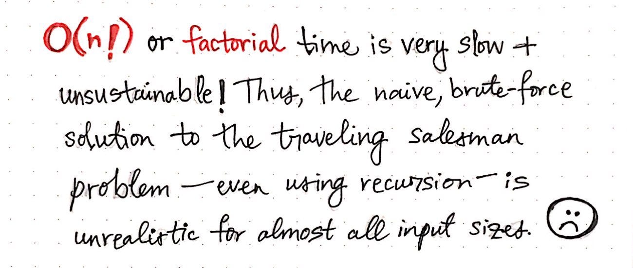
O(n!) runtime is unsustainable.

We have seen quite a few different forms of Big O Notation throughout this series, including the good and the bad. So, where do factorial algorithms fit into this narrative?

If constant, logarithmic, and linear time are good, and quadratic and exponential time are bad, there is only one thing left to explore: the ugly. Factorial algorithms are exactly that: the ugly.

For an algorithm that runs in factorial, or O(n!) time, any operations that need to run will end up taking n! more time in relation to the data that is being operated upon, or the input data set.

Okay, but what does this actually mean? Well, let’s look at how a factorial algorithm compares to all the other forms of Big O Notation that we’re already familiar with.

 

Factorial time is super slow and inefficient as input size grows

We’ll notice almost immediately that algorithms that grow in factorial time are super slow and ineffcient as input size grows. For example, we’ll see that even a slight increase in the number of elements to be operated upon by a factorial algorithm causes it to shoot up in the number of operations required to run. If we compare this to linearithmic, linear, or even just quadratic time algorithms— which are still pretty bad in their own right — we’ll see that factorial algorithms are obsecenely terrible in comparison!

All of this is to say: our first approach to solving TSP using brute-force recursion is probably not the best solution. Yes, it works, but it’s probably not as “right” as it could be; it could stand to be improved, and surely could be made more elegant. And, of course, it is not fast — at all!

 

Using brute-force takes a top-down approach to solving TSP.

So, how can we improve upon this first attempt that we made?

Well, if we think back to our foray into dynamic programming (DP), we’ll remember that there is more than one approach when it comes to solving a DP problem. In our initial stab at this problem, we attempted to solve TSP using a kind of top down approach: we started with a large, complex problem, and broke it down into smaller parts. Then, when we got down to our base case, and expanded the problem down to its smallest possible parts, we used recursion to build up all the possible paths that our traveling salesman could take, which allowed us to choose the best (the shortest) permutation of all the paths that we had found.

In the process, we figured out one way to solve the traveling salesman problem. But what if we approached it a different manner? What would happen if we took our top down approach and turned it upside down?

There’s only one way to find out — we have to try it out!

Turning TSP on its head

If we look at our top down methodology from last week, we’ll see that we have enumerated through all of the permutations of paths — that is to say, we have brute-forced our way to determine every single route that our traveling salesman could take.

 

The brute-force approach to solving TSP.

This methodology isn’t particularly elegant, is kind of messy, and, as we have already determined, will simply never scale as our input size grows. But ignoring all of those issues for a moment, let’s just take a look at this “tree” of recursive function calls once again.

 

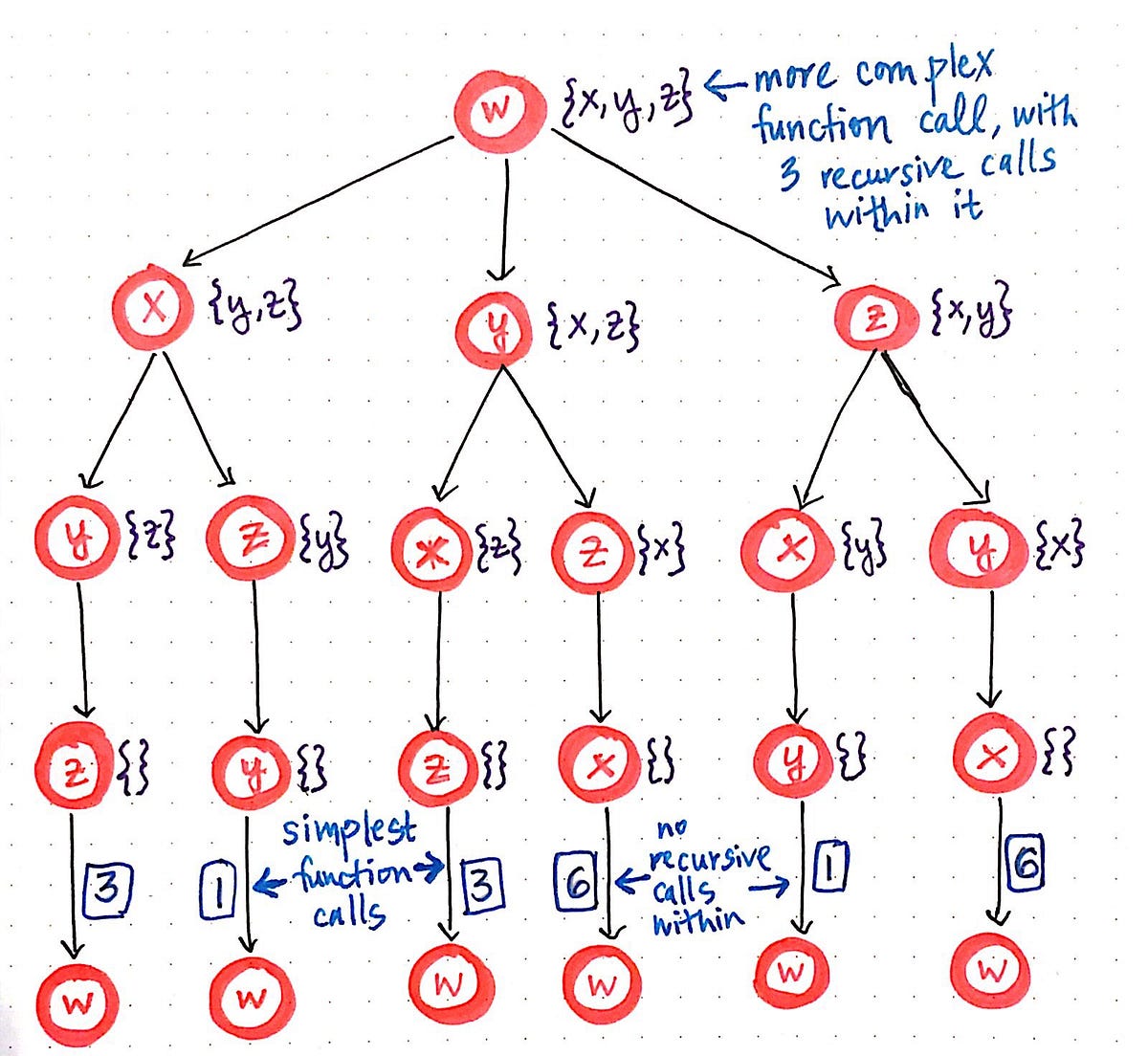
Rethinking the brute-force approach by identifying the simplest problem, or function call.

On second glance, we’ll notice that there is something interesting going on here: we’re starting with the more complex function call initially, and then, from within that, we are invoking three recursive function calls from within it. Each of those three recursive function calls spins off two more recursive calls of its own, which creates the third level of this function call “tree”. This is, of course, keeping in tune with our working definition of a top down approach: starting with the largest problem first, and breaking it down into its smallest parts. But, now that we can see the smallest parts more obviously, we can change our approach from a top down method to a bottom up method.

We’ll recall that a bottom up dynamic programming approach starts with the smallest possible subproblems, figures out a solution to them, and then slowly builds itself up to solve the larger, more complicated subproblem. In the context of our “function call tree”, the smallest possible subproblem are the smallest possible function calls. We’ll see that the smallest function calls are the simplest ones — the ones that have no recursive calls within them. In our case, these are the function calls at the very bottom of our “function call tree”, which lead back to our starting node, node w, which is the city that our traveling salesman is “starting” from, and will inevitably have to “end” up at.

Now that we’ve identified the smallest possible subproblems, we can turn TSP on its head. We’ll flip our top down approach to this problem and, instead, use a bottom up approach here. Let’s start with our three simplest function calls.

 

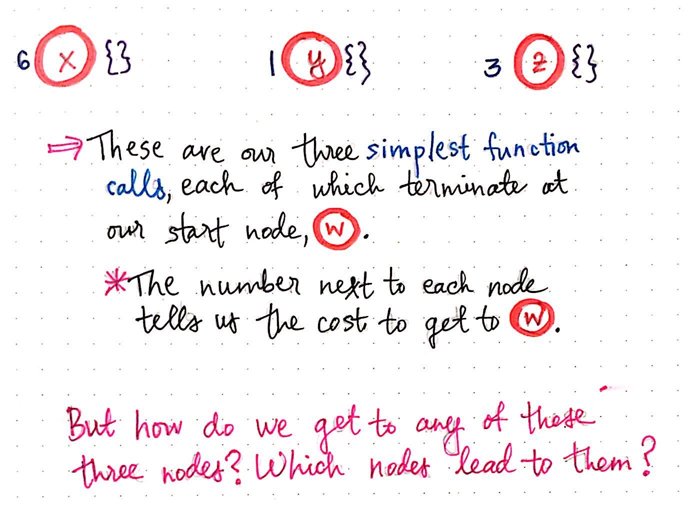
Flipping TSP on its head, part 1.

We’ll see that each of these calls connects back to w, as we would expect. Recall that we’re using a list notationto keep track of the nodes that we can navigate to. Since we’re dealing with the smallest possible subproblem(s), there is nowhere that we can navigate to from these nodes; instead, all we can do is go back to our starting node, w. This is why each of the lists for these three subproblems is empty ({}).

However, we do need to keep track of cost and distance here, since inevitably, we’re still going to have to find the shortest path for our traveling salesman, regardless of whether we’re using a top down or bottom up approach. Thus, we’re going to have to keep track of the distance between nodes as we build up our “bottom up” tree. In the image above, we’ll see that we have the values 6, 1, and 3 next to nodes x, y, and z, respectively. These number represent the distance to get from each node back to the origin node, w.

When we first tried to solve TSP, we used an adjacency matrix to help us keep track of the distances between nodes in our graph. We’ll lean on our adjacency matrix in this approach yet again.

However, in our bottom up approach, we’ll use it to enumerate all the function calls that lead to one another. This is strikingly different than our top down approach, when we were using our adjacency matrix to help us enumerate all the possible paths. In our bottom up approach, we’re trying to be a bit more elegant about how we do things, so we’re aiming to not enumerate more than we need to! This will make more sense as we go on, but it’s important to note the difference between enumerating paths versus enumerating function calls.

So, what would the second level of our function call “tree” look like? Well, the question that we’re trying to answer for each of our smallest possible subproblems here is this:

If we are at the simplest possible version of this function call and cannot call anything recursively from within this function, what other function could possibly call this one?

 

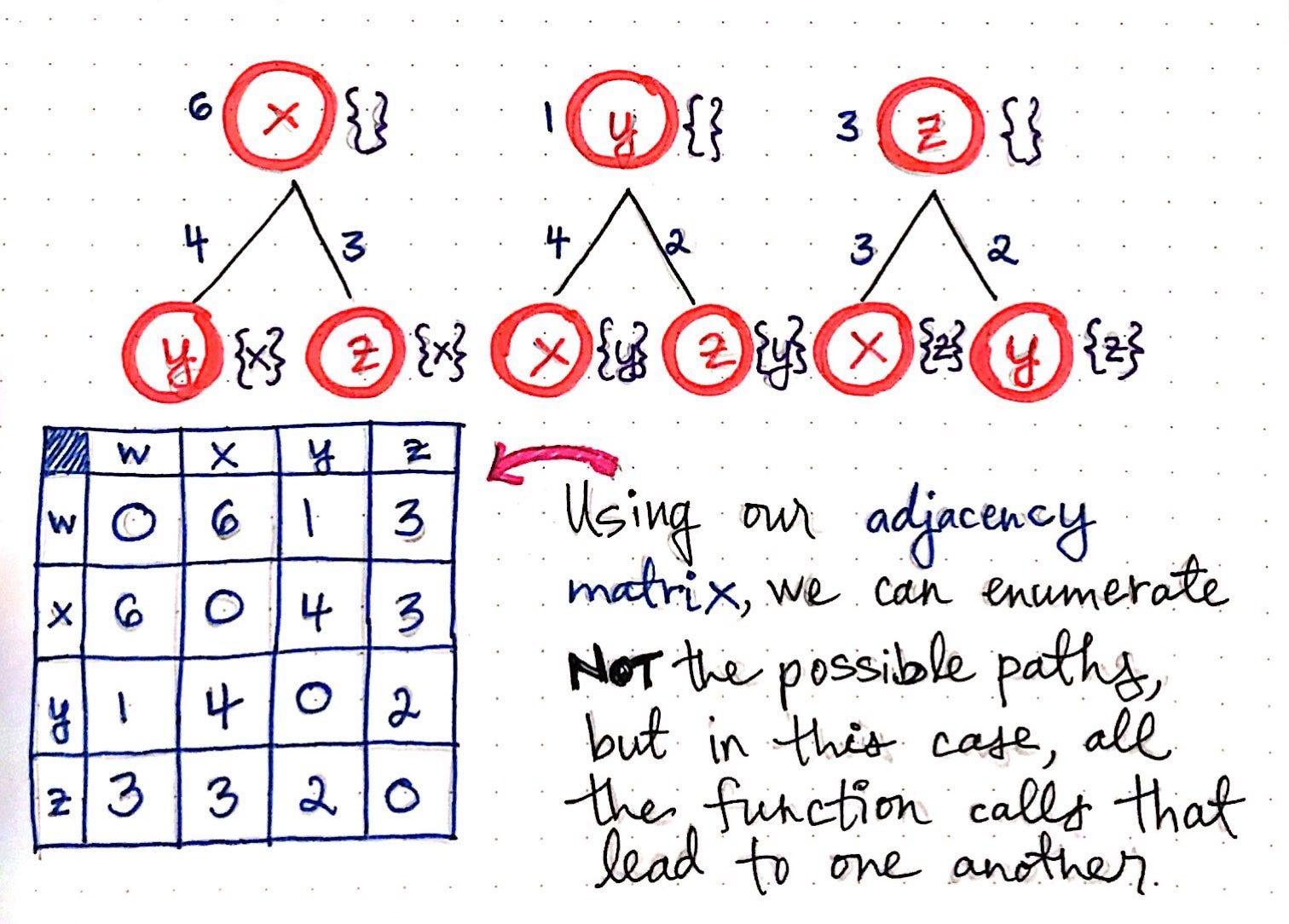
Flipping TSP on its head, part 2.

Another way of thinking about it is in terms of nodes. Ultimately, we’re trying to determine which possible nodes would allow us to get to the node that we’re looking at. So, in the case of node x, the only way to get to node x would potentially be node y or node z. Remember that we’re using a bottom up approach here, so we’re almost retracing our steps backwards, starting at the end, and working our way back through the circle.

Notice, again, that we’re keeping track of the cost/distance from each of these nodes to the next. We’re going to need them pretty soon!

Again, we can expand this function call “tree” a bit more to add another level. Remember, we’re trying to answer the question: what other function could possibly call this function that we cannot expand any further?

 

Flipping TSP on its head, part 3.

In the drawing depicted here, we’ll see what this actually looks like in practice. For example, looking at the leftmost branch of this function call “tree”, we’ll notice that the only possible function call that will allow us to get to an empty node x is from either node y or node z, where the set contains only a possible “next” node of x, like so: {x}. For both node y and z in the leftmost subtree, we’ll see that the only possible way to get to y is from node z, when the set contains both x and y (or {x, y}). Similarly, the only possible way to get to z is from node y, when the set contains both x and z (or {x, z}).

This is a visualization exemplifies what we mean when we say that we are enumerating function calls rather than enumerating potential paths. As we continue to determine all the possible function calls that allow us to call other functions from within them, something starts to become very obvious: we have some overlapping subproblems here!

We’ll notice that there are two function calls that are instances of z when its set contains both x and y (or {x, y}), which is highlighted in yellow. Similarly, there are two function calls that are instances of y when its set contains both x and z (or {x, z}), highlighted in pink. Finally, we’ll see two function calls that are instances of x when its set contains both y and z (or {y, z}), highlighted in green.

Dynamic programming is all about identifying repeated work and being smarter and more efficient with our approach so that we don’t actually have to repeat ourselves! So, let’s cut out this repetition and use some dynamic programming to make things a little better for our traveling salesman.

Dynamic programming to the salesman’s rescue

Now that we’ve identified our overlapping and recurring subproblems, there’s only one thing left to do: eliminate the repetition, of course!

 

Flipping TSP on its head, part 4.

Using our function call “tree”, we can rearrange some of our function calls so that we’re not actually repeating ourselves in level three of this tree.

We can do this by cutting down our repeated subproblems so that they only show up once. Then, we’ll reconfigure the bottom level of our tree so that it is still accurate, but also that we each function call show up once, not twice.

Now it starts to become apparent how the bottom up approach is different than our top down method from before.

We’ll see that we no longer need to do the work of generating that entire bottom level of our function call “tree” in order to figure out all o the recursive function calls. Nor do we need to determine all the possible paths that our traveling salesman could take by using brute force. Instead, we’re enumerating through function calls, finding the repeated ones, and condensing our “tree” of function calls as we continue to build it.

Once we’ve eliminated the repeated subproblems, we can do the work of actually finding the shortest path. Remember that we will need to use our adjacency matrix to figure out the distance between one node to another. But, we’ll also notice that we’re not having to repeat ourselves nearly as much because we won’t see the same numbers appear too many times as we sum them up.

In the illustration shown below, each of the function calls that allow our salesman to traverse from one node to another has a number (the cost or distance) associated with it. As we continue down this tree, we’ll sum up the cost of each set of function calls. For example, if we choose the function calls that lead from w <- x <- y <- z, we’ll sum up the cost between these nodes, which amounts to 6 + 4 + 2 = 12.

 

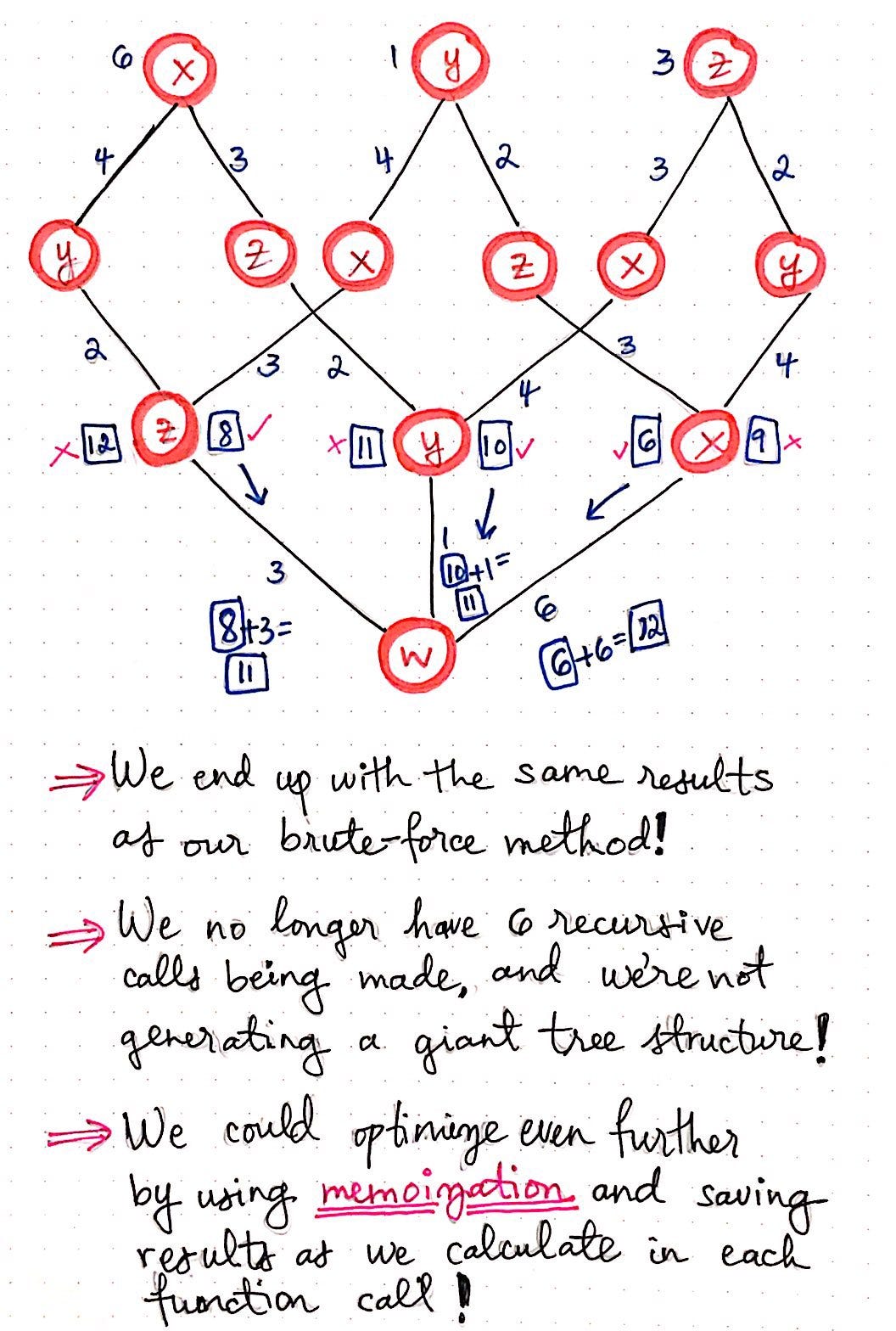
Flipping TSP on its head, part 5.

When we get down to the third level of our function call “tree”, we’ll see that we have two numbers that we can choose from. Recall that we had a similar scenario happen to us in our top down approach last week: we had two different paths with two different costs/distances to choose from. We ended up choosing the smaller of the two cost, since we’re trying to find the shortest path for our salesman. In this case, we have two different function calls, with two different costs/distances to choose from. Again, we’ll choose the smaller of the two costs, since we’re still trying to find the shortest path here, too!

Eventually, as we continue sum the distances/costs, we’ll see that we ended up witht he exact same results as our brute-force method from last week. The shortest cost for our traveling salesman is going to be 11, and there are two possible paths that would allow for them to achieve that lowest cost. However, using the bottom up approach, we’ve optimized our TSP algorithm, since we no longer have six recursive calls being made in this method. Furthermore, we’re also not generating as big of a tree structure! If we think back to when we were first introduced to dynamic programming, we’ll recall that we could also use memoization and save the results of our function calls as we calculate them, optimizing our solution even further.

 

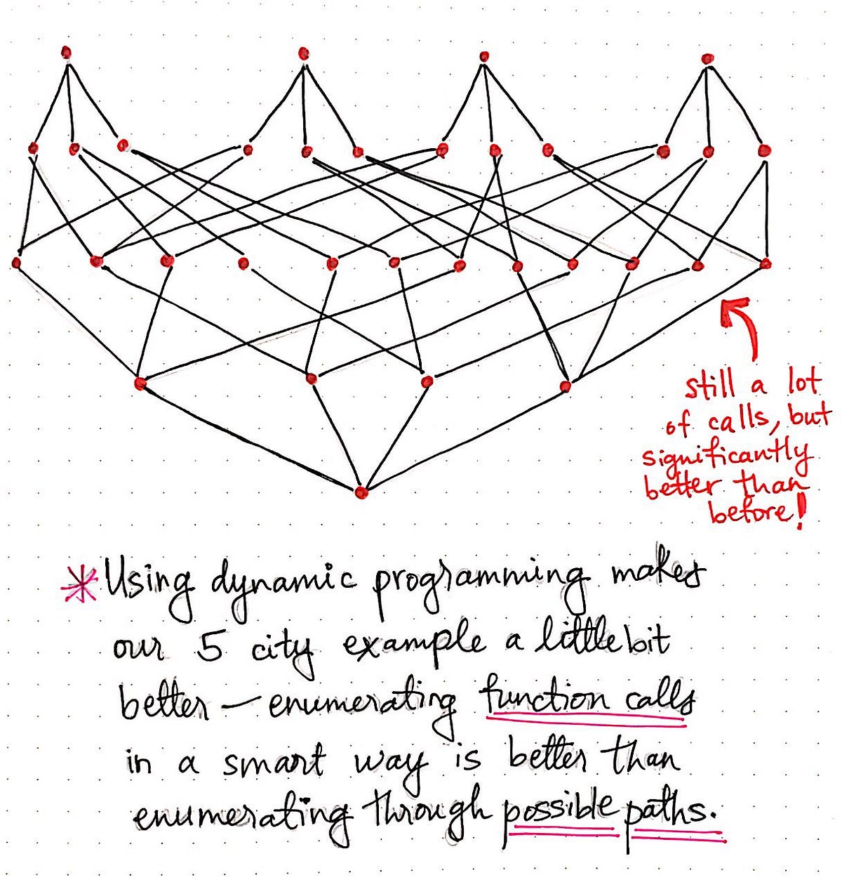
Using dynamic programming makes our 5 city example a little faster.

Okay, so we started down this path in an effort to take the next step in the adage of “Make it work, make it right, make it fast.”

We have arguably made our workable solution much better, and certainly more elegant, and far less repetitive. The illustration shown here exemplifies how the bottom up DP approach would scale for a traveling salesman problem where the salesman has to visit five cities instead of four. We’ll see that we’re still making a lot of calls, but our function call “tree” is a bit slimmer and significantly better than before.

By using dynamic programming, we’ve made our solution for the traveling salesman problem just a little bit better by choosing to smartly enumerate function calls rather than brute-force our way through every single possible path that our salesman could take.

The only question we have to answer now is, of course, how does the runtime of this method compare to our ugly factorial, O(n!) runtime from earlier?

Well, as it turns out, the bottom up approach that we’ve been exploring here is really the foundations of something called the Held-Karp algorithm, which is also often referred to as the Bellman-Held-Karp algorithm. This algorithm was derived in 1962, by both Michael Held and Richard M. Karp as well as Richard Bellman, who was working independently on his own related research at the time.

 

The Held-Karp algorithm uses dynamic programming to approach TSP.

The Held-Karp algorithm actually proposed the bottom up dynamic programming approach as a solution to improving the brute-force method of solving the traveling salesman problem. Bellman, Held, and Karp’s algorithm was determined to run in exponential time, since it still does a bulk of the work of enumerating through all the potential sets of function calls that are possible. The exponential runtime of the Held-Karp algorithm is still not perfect — it’s far from it, in fact! But, it’s not as ugly as a factorial algorithm, and it’s still an improvement.

And, to be honest, I’m sure the traveling salesman would be happy to take whatever he could get.

Resources

The traveling salesman problem has been written about, researched, and taught extensively. As it turns out, there are many different approaches when it comes to attempting to solve it, and the Held-Karp algorithm is just one of them. If you want to dig deeper into this particular topic, here are some good places to start.