改善深层神经网络-week3编程题（Tensorflow 实现手势识别 ）

TensorFlow Tutorial

• Initialize variables
• Start your own session
• Train algorithms
• Implement a Neural Network

1. Exploring the Tensorflow Library

To start, you will import the library:

import math
import numpy as np
import h5py
import matplotlib.pyplot as plt
import tensorflow as tf
from tensorflow.python.framework import ops
from tf_utils import load_dataset, random_mini_batches, convert_to_one_hot, predict
%matplotlib inline
np.random.seed(1)

Now that you have imported the library, we will walk you through its different applications. You will start with an example, where we compute for you the loss of one training example.

\[loss = \mathcal{L}(\hat{y}, y) = (\hat y^{(i)} - y^{(i)})^2 \tag{1}
\]

y_hat = tf.constant(36, name='y_hat')            # Define y_hat constant. Set to 36.
y = tf.constant(39, name='y')                    # Define y. Set to 39
loss = tf.Variable((y - y_hat)**2, name='loss')  # Create a variable for the loss
init = tf.global_variables_initializer()         # When init is run later (session.run(init)),
                                                 # the loss variable will be initialized and ready to be computed
with tf.Session() as session:                    # Create a session and print the output
    session.run(init)                            # Initializes the variables
    print(session.run(loss))                     # Prints the loss

Writing and running programs in TensorFlow has the following steps:

1. Create Tensors (variables) that are not yet executed/evaluated.
2. Write operations between those Tensors.
3. Initialize your Tensors.
4. Create a Session.
5. Run the Session. This will run the operations you'd written above.

1.1 - Linear function

Lets start this programming exercise by computing the following equation: \(Y = WX + b\), where \(W\) and \(X\) are random matrices and b is a random vector.

Exercise: Compute \(WX + b\) where \(W, X\), and \(b\) are drawn from a random normal distribution. W is of shape (4, 3), X is (3,1) and b is (4,1). As an example, here is how you would define a constant X that has shape (3,1):

X = tf.constant(np.random.randn(3,1), name = "X")

You might find the following functions helpful:

• tf.matmul(..., ...) to do a matrix multiplication
• tf.add(..., ...) to do an addition
• np.random.randn(...) to initialize randomly

# GRADED FUNCTION: linear_function
def linear_function():
    """
    Implements a linear function:
            Initializes W to be a random tensor of shape (4,3)
            Initializes X to be a random tensor of shape (3,1)
            Initializes b to be a random tensor of shape (4,1)
    Returns:
    result -- runs the session for Y = WX + b
    """
    np.random.seed(1)
    ### START CODE HERE ### (4 lines of code)
    W = tf.constant(np.random.randn(4, 3), name='W')
    X = tf.constant(np.random.randn(3, 1), name='X')
    b = tf.constant(np.random.randn(4, 1), name='b')
    Y = tf.add(tf.matmul(W, X), b)
    ### END CODE HERE ### 
    # Create the session using tf.Session() and run it with sess.run(...) on the variable you want to calculate
    ### START CODE HERE ###
    sess = tf.Session()
    result = sess.run(Y)
    ### END CODE HERE ###
    # close the session
    sess.close()
    return result

1.2 - Computing the sigmoid

Great! You just implemented a linear function. Tensorflow offers a variety of commonly used neural network functions like tf.sigmoid and tf.softmax. For this exercise lets compute the sigmoid function of an input.

You will do this exercise using a placeholder variable x. When running the session, you should use the feed dictionary to pass in the input z. In this exercise, you will have to (i) create a placeholder x, (ii) define the operations needed to compute the sigmoid using tf.sigmoid, and then (iii) run the session.

** Exercise **: Implement the sigmoid function below. You should use the following:

• tf.placeholder(tf.float32, name = "...")
• tf.sigmoid(...)
• sess.run(..., feed_dict = {x: z})

Note that there are two typical ways to create and use sessions in tensorflow:

Method 1:

sess = tf.Session()
# Run the variables initialization (if needed), run the operations
result = sess.run(..., feed_dict = {...})
sess.close() # Close the session

Method 2:

with tf.Session() as sess:
    # run the variables initialization (if needed), run the operations
    result = sess.run(..., feed_dict = {...})
    # This takes care of closing the session for you :)

print ("sigmoid(0) = " + str(sigmoid(0)))
print ("sigmoid(12) = " + str(sigmoid(12)))

输出:

sigmoid(0) = 0.5

sigmoid(12) = 0.9999942

**To summarize, you how know how to**:
1. Create placeholders
2. Specify the computation graph corresponding to operations you want to compute
3. Create the session
4. Run the session, using a feed dictionary if necessary to specify placeholder variables' values.

1.3 - Computing the Cost

You can also use a built-in function to compute the cost of your neural network. So instead of needing to write code to compute this as a function of \(a^{[2](i)}\) and \(y^{(i)}\) for i=1...m:

\[J = - \frac{1}{m} \sum_{i = 1}^m \large ( \small y^{(i)} \log a^{ [2] (i)} + (1-y^{(i)})\log (1-a^{ [2] (i)} )\large )\small\tag{2}
\]

you can do it in one line of code in tensorflow!

Exercise: Implement the cross entropy loss. The function you will use is:

• tf.nn.sigmoid_cross_entropy_with_logits(logits = ..., labels = ...)

Your code should input z, compute the sigmoid (to get a) and then compute the cross entropy cost \(J\). All this can be done using one call to tf.nn.sigmoid_cross_entropy_with_logits, which computes

\[- \frac{1}{m} \sum_{i = 1}^m \large ( \small y^{(i)} \log \sigma(z^{[2](i)}) + (1-y^{(i)})\log (1-\sigma(z^{[2](i)})\large )\small\tag{2}
\]

# GRADED FUNCTION: cost
def cost(logits, labels):
    """
    Computes the cost using the sigmoid cross entropy
    
    Arguments:
    logits -- vector containing z, output of the last linear unit (before the final sigmoid activation)
    labels -- vector of labels y (1 or 0) 
    Note: What we've been calling "z" and "y" in this class are respectively called "logits" and "labels"
    in the TensorFlow documentation. So logits will feed into z, and labels into y.
    
    Returns:
    cost -- runs the session of the cost (formula (2))
    """
    ### START CODE HERE ###
    z = tf.placeholder(tf.float32, name='z')
    y = tf.placeholder(tf.float32, name='y')
    # Use the loss function (approx. 1 line)
    cost = tf.nn.sigmoid_cross_entropy_with_logits(logits=z, labels=y)
    # Create a session (approx. 1 line). See method 1 above.
    sess = tf.Session()
    # Run the session (approx. 1 line).
    cost = sess.run(cost, feed_dict={z: logits, y:labels})
    # Close the session (approx. 1 line). See method 1 above.
    sess.close()
    ### END CODE HERE ###
    return cost

logits = sigmoid(np.array([0.2,0.4,0.7,0.9]))
cost = cost(logits, np.array([0,0,1,1]))
print ("cost = " + str(cost))

cost = [ 1.00538719 1.03664088 0.41385433 0.39956614]

1.4 - Using One Hot encodings

Many times in deep learning you will have a y vector with numbers ranging from 0 to C-1, where C is the number of classes. If C is for example 4, then you might have the following y vector which you will need to convert as follows:

This is called a "one hot" encoding, because in the converted representation exactly one element of each column is "hot" (meaning set to 1). To do this conversion in numpy, you might have to write a few lines of code. In tensorflow, you can use one line of code:

• tf.one_hot(labels, depth, axis)

Exercise: Implement the function below to take one vector of labels and the total number of classes \(C\), and return the one hot encoding. Use tf.one_hot() to do this.

# GRADED FUNCTION: one_hot_matrix
def one_hot_matrix(labels, C):
    """
    Creates a matrix where the i-th row corresponds to the ith class number and the jth column
                     corresponds to the jth training example. So if example j had a label i. Then entry (i,j)
                     will be 1. 
    Arguments:
    labels -- vector containing the labels
    C -- number of classes, the depth of the one hot dimension
    Returns:
    one_hot -- one hot matrix
    """
    ### START CODE HERE ###
    # Create a tf.constant equal to C (depth), name it 'C'. (approx. 1 line)
    C = tf.constant(C, name='C')
    # Use tf.one_hot, be careful with the axis (approx. 1 line)
    one_hot_matrix = tf.one_hot(indices=labels, depth=C, axis=0)
    # Create the session (approx. 1 line)
    sess = tf.Session()
    # Run the session (approx. 1 line)
    one_hot = sess.run(one_hot_matrix)
    # Close the session (approx. 1 line). See method 1 above.
    sess.close()
    ### END CODE HERE ###
    return one_hot

输出：

labels = np.array([1,2,3,0,2,1])
one_hot = one_hot_matrix(labels, C = 4)
print ("one_hot = " + str(one_hot))

1.5 - Initialize with zeros and ones

Now you will learn how to initialize a vector of zeros and ones. The function you will be calling is tf.ones(). To initialize with zeros you could use tf.zeros() instead. These functions take in a shape and return an array of dimension shape full of zeros and ones respectively.

Exercise: Implement the function below to take in a shape and to return an array (of the shape's dimension of ones).

• tf.ones(shape)

# GRADED FUNCTION: ones
def ones(shape):
    """
    Creates an array of ones of dimension shape
    Arguments:
    shape -- shape of the array you want to create
    Returns:
    ones -- array containing only ones
    """
    ### START CODE HERE ###
    # Create "ones" tensor using tf.ones(...). (approx. 1 line)
    ones = tf.ones(shape)
    # Create the session (approx. 1 line)
    sess = tf.Session()
    # Run the session to compute 'ones' (approx. 1 line)
    ones = sess.run(ones)
    # Close the session (approx. 1 line). See method 1 above.
    sess.close()
    ### END CODE HERE ###
    return ones

测试：

print ("ones = " + str(ones([3])))

2 - Building your first neural network in tensorflow

In this part of the assignment you will build a neural network using tensorflow. Remember that there are two parts to implement a tensorflow model:

• Create the computation graph
• Run the graph

Let's delve into the problem you'd like to solve!

2.0 - Problem statement: SIGNS Dataset

手势数字识别

• Training set: 1080 pictures (64 by 64 pixels) of signs representing numbers from 0 to 5 (180 pictures per number).
• Test set: 120 pictures (64 by 64 pixels) of signs representing numbers from 0 to 5 (20 pictures per number).

Note that this is a subset of the SIGNS dataset. The complete dataset contains many more signs.

Here are examples for each number, and how an explanation of how we represent the labels. These are the original pictures, before we lowered the image resolutoion to 64 by 64 pixels.

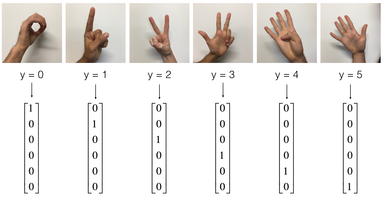
Figure 1: SIGNS dataset

Run the following code to load the dataset.

# Loading the dataset
X_train_orig, Y_train_orig, X_test_orig, Y_test_orig, classes = load_dataset()

Change the index below and run the cell to visualize some examples in the dataset.

# Example of a picture
index = 0
plt.imshow(X_train_orig[index])
print ("y = " + str(np.squeeze(Y_train_orig[:, index])))

y = 4

像往常那样flatten图像数据，并且用 x /= 255. 正则化数据。除此之外，你需要转换每个数字标签，为一个 one-hot向量，如 Figure 1.

# Flatten the training and test images
X_train_flatten = X_train_orig.reshape(X_train_orig.shape[0], -1).T
X_test_flatten = X_test_orig.reshape(X_test_orig.shape[0], -1).T
# Normalize image vectors
X_train = X_train_flatten/255.
X_test = X_test_flatten/255.
# Convert training and test labels to one hot matrices
Y_train = convert_to_one_hot(Y_train_orig, 6)
Y_test = convert_to_one_hot(Y_test_orig, 6)
print ("number of training examples = " + str(X_train.shape[1]))
print ("number of test examples = " + str(X_test.shape[1]))
print ("X_train shape: " + str(X_train.shape))
print ("Y_train shape: " + str(Y_train.shape))
print ("X_test shape: " + str(X_test.shape))
print ("Y_test shape: " + str(Y_test.shape))

number of training examples = 1080

number of test examples = 120

X_train shape: (12288, 1080)

Y_train shape: (6, 1080)

X_test shape: (12288, 120)

Y_test shape: (6, 120)

Note that 12288 comes from \(64 \times 64 \times 3\). Each image is square, 64 by 64 pixels, and 3 is for the RGB colors. Please make sure all these shapes make sense to you before continuing.

Your goal is to build an algorithm capable of recognizing a sign with high accuracy. To do so, you are going to build a tensorflow model that is almost the same as one you have previously built in numpy for cat recognition (but now using a softmax output).

The model is LINEAR -> RELU -> LINEAR -> RELU -> LINEAR -> SOFTMAX. (要输出多个分类）

2.1 - Create placeholders

Your first task is to create placeholders for X and Y. This will allow you to later pass your training data in when you run your session.

Exercise: Implement the function below to create the placeholders in tensorflow.

# GRADED FUNCTION: create_placeholders
def create_placeholders(n_x, n_y):
    """
    Creates the placeholders for the tensorflow session.
    Arguments:
    n_x -- scalar, size of an image vector (num_px * num_px = 64 * 64 * 3 = 12288)
    n_y -- scalar, number of classes (from 0 to 5, so -> 6)
    Returns:
    X -- placeholder for the data input, of shape [n_x, None] and dtype "float"
    Y -- placeholder for the input labels, of shape [n_y, None] and dtype "float"
    Tips:
    - You will use None because it let's us be flexible on the number of examples you will for the placeholders.
      In fact, the number of examples during test/train is different.
    """
    ### START CODE HERE ### (approx. 2 lines)
    X = tf.placeholder(tf.float32, shape=[n_x, None], name='X')
    Y = tf.placeholder(tf.float32, shape=[n_y, None], name='Y')
    ### END CODE HERE ###
    return X, Y

X, Y = create_placeholders(12288, 6)
print ("X = " + str(X))
print ("Y = " + str(Y))

X = Tensor("X_1:0", shape=(12288, ?), dtype=float32)

Y = Tensor("Y:0", shape=(6, ?), dtype=float32)

2.2 - Initializing the parameters

initialize the parameters in tensorflow.

Exercise: 在TensorFlow中初始化参数. 用 Xavier Initialization 对 weights 并且用 Zero Initialization for biases. As an example, to help you, for W1 and b1 you could use:

W1 = tf.get_variable("W1", [25,12288], initializer = tf.contrib.layers.xavier_initializer(seed = 1))
b1 = tf.get_variable("b1", [25,1], initializer = tf.zeros_initializer())

Please use seed = 1 to make sure your results match ours.

# GRADED FUNCTION: initialize_parameters
def initialize_parameters():
    """
    Initializes parameters to build a neural network with tensorflow. The shapes are:
                        W1 : [25, 12288]
                        b1 : [25, 1]
                        W2 : [12, 25]
                        b2 : [12, 1]
                        W3 : [6, 12]
                        b3 : [6, 1]
    Returns:
    parameters -- a dictionary of tensors containing W1, b1, W2, b2, W3, b3
    """
    tf.set_random_seed(1)                   # so that your "random" numbers match ours
    ### START CODE HERE ### (approx. 6 lines of code)
    W1 = tf.get_variable("W1", [25, 12288], initializer=tf.contrib.layers.xavier_initializer(seed=1))
    b1 = tf.get_variable("b1", [25, 1], initializer=tf.zeros_initializer())
    W2 = tf.get_variable("W2", [12, 25], initializer=tf.contrib.layers.xavier_initializer(seed=1))
    b2 = tf.get_variable("b2", [12, 1], initializer=tf.zeros_initializer())
    W3 = tf.get_variable("W3", [6, 12], initializer=tf.contrib.layers.xavier_initializer(seed=1))
    b3 = tf.get_variable("b3", [6, 1], initializer=tf.zeros_initializer())
    ### END CODE HERE ###
    parameters = {"W1": W1,
                  "b1": b1,
                  "W2": W2,
                  "b2": b2,
                  "W3": W3,
                  "b3": b3}
    return parameters

tf.reset_default_graph()
with tf.Session() as sess:
    parameters = initialize_parameters()
    print("W1 = " + str(parameters["W1"]))
    print("b1 = " + str(parameters["b1"]))
    print("W2 = " + str(parameters["W2"]))
    print("b2 = " + str(parameters["b2"]))

W1 = <tf.Variable 'W1:0' shape=(25, 12288) dtype=float32_ref>

b1 = <tf.Variable 'b1:0' shape=(25, 1) dtype=float32_ref>

W2 = <tf.Variable 'W2:0' shape=(12, 25) dtype=float32_ref>

b2 = <tf.Variable 'b2:0' shape=(12, 1) dtype=float32_ref>

2.3 - Forward propagation in tensorflow

implement the forward propagation module in tensorflow. The function will take in a dictionary of parameters and it will complete the forward pass. The functions you will be using are:

• tf.add(...,...) to do an addition
• tf.matmul(...,...) to do a matrix multiplication(矩阵乘法)
• tf.nn.relu(...) to apply the ReLU activation

Question: Implement the forward pass of the neural network. We commented for you the numpy equivalents so that you can compare the tensorflow implementation to numpy. It is important to note that the forward propagation stops at z3. The reason is that in tensorflow the last linear layer output is given as input to the function computing the loss. Therefore, you don't need a3!

# GRADED FUNCTION: forward_propagation
def forward_propagation(X, parameters):
    """
    Implements the forward propagation for the model: LINEAR -> RELU -> LINEAR -> RELU -> LINEAR -> SOFTMAX
    Arguments:
    X -- input dataset placeholder, of shape (input size, number of examples)
    parameters -- python dictionary containing your parameters "W1", "b1", "W2", "b2", "W3", "b3"
                  the shapes are given in initialize_parameters
    Returns:
    Z3 -- the output of the last LINEAR unit
    """
    # Retrieve the parameters from the dictionary "parameters"
    W1 = parameters['W1']
    b1 = parameters['b1']
    W2 = parameters['W2']
    b2 = parameters['b2']
    W3 = parameters['W3']
    b3 = parameters['b3']
    ### START CODE HERE ### (approx. 5 lines)              # Numpy Equivalents:
    Z1 = tf.add(tf.matmul(W1, X), b1)                      # Z1 = np.dot(W1, X) + b1
    A1 = tf.nn.relu(Z1)                                    # A1 = relu(Z1)
    Z2 = tf.add(tf.matmul(W2, A1), b2)                     # Z2 = np.dot(W2, a1) + b2
    A2 = tf.nn.relu(Z2)                                    # A2 = relu(Z2)
    Z3 = tf.add(tf.matmul(W3, A2), b3)                     # Z3 = np.dot(W3,Z2) + b3
    ### END CODE HERE ###
    return Z3

tf.reset_default_graph()
with tf.Session() as sess:
    X, Y = create_placeholders(12288, 6)
    parameters = initialize_parameters()
    Z3 = forward_propagation(X, parameters)
    print("Z3 = " + str(Z3))

2.4 - Compute cost

As seen before, it is very easy to compute the cost using:

tf.reduce_mean(tf.nn.softmax_cross_entropy_with_logits(logits = ..., labels = ...))

Question: Implement the cost function below.

• It is important to know that the "logits" and "labels" inputs of tf.nn.softmax_cross_entropy_with_logits are expected to be of shape (number of examples, num_classes). We have thus transposed Z3 and Y for you.
• Besides, tf.reduce_mean basically does the summation over the examples.

# GRADED FUNCTION: compute_cost 
def compute_cost(Z3, Y):
    """
    Computes the cost
    Arguments:
    Z3 -- output of forward propagation (output of the last LINEAR unit), of shape (6, number of examples)
    Y -- "true" labels vector placeholder, same shape as Z3
    Returns:
    cost - Tensor of the cost function
    """
    # to fit the tensorflow requirement for tf.nn.softmax_cross_entropy_with_logits(...,...)
    logits = tf.transpose(Z3)   # 转置
    labels = tf.transpose(Y)
    ### START CODE HERE ### (1 line of code)
    # tf.reduce_mean 函数用于计算张量tensor沿着指定的数轴（tensor的某一维度）上的的平均值，
    # 主要用作降维或者计算tensor（图像）的平均值。
    cost = tf.reduce_mean(tf.nn.softmax_cross_entropy_with_logits(logits=logits,
                                                                 labels=labels))
    ### END CODE HERE ###
    return cost

tf.reset_default_graph()
with tf.Session() as sess:
    X, Y = create_placeholders(12288, 6)
    parameters = initialize_parameters()
    Z3 = forward_propagation(X, parameters)
    cost = compute_cost(Z3, Y)
    print("cost = " + str(cost))

cost = Tensor("Mean:0", shape=(), dtype=float32)

2.5 - Backward propagation & parameter updates

All the backpropagation and the parameters update is taken care of in 1 line of code.

After you compute the cost function. You will create an "optimizer" object. 选择优化函数(optimization) 和 learning rate 最小化代价。

For instance, for gradient descent the optimizer would be:

optimizer = tf.train.GradientDescentOptimizer(learning_rate = learning_rate).minimize(cost)

To make the optimization you would do:

_ , c = sess.run([optimizer, cost], feed_dict={X: minibatch_X, Y: minibatch_Y})

This computes the backpropagation by passing through the tensorflow graph in the reverse order. From cost to inputs.

Note When coding, we often use _ as a "throwaway" variable to store values that we won't need to use later. Here, _ takes on the evaluated value of optimizer, which we don't need (and c takes the value of the cost variable).

2.6 - Building the model

Now, you will bring it all together!

Exercise: Implement the model. You will be calling the functions you had previously implemented.

def model(X_train, Y_train, X_test, Y_test, learning_rate = 0.0001,
          num_epochs = 1500, minibatch_size = 32, print_cost = True):
    """
    Implements a three-layer tensorflow neural network: LINEAR->RELU->LINEAR->RELU->LINEAR->SOFTMAX.
    Arguments:
    X_train -- training set, of shape (input size = 12288, number of training examples = 1080)
    Y_train -- test set, of shape (output size = 6, number of training examples = 1080)
    X_test -- training set, of shape (input size = 12288, number of training examples = 120)
    Y_test -- test set, of shape (output size = 6, number of test examples = 120)
    learning_rate -- learning rate of the optimization
    num_epochs -- number of epochs of the optimization loop
    minibatch_size -- size of a minibatch
    print_cost -- True to print the cost every 100 epochs
    Returns:
    parameters -- parameters learnt by the model. They can then be used to predict.
    """
    ops.reset_default_graph()                         # to be able to rerun the model without overwriting tf variables
    tf.set_random_seed(1)                             # to keep consistent results
    seed = 3                                          # to keep consistent results
    (n_x, m) = X_train.shape                          # (n_x: input size, m : number of examples in the train set)
    n_y = Y_train.shape[0]                            # n_y : output size
    costs = []                                        # To keep track of the cost
    # Create Placeholders of shape (n_x, n_y)
    ### START CODE HERE ### (1 line)
    X, Y = create_placeholders(n_x, n_y)
    ### END CODE HERE ###
    # Initialize parameters
    ### START CODE HERE ### (1 line)
    parameters = initialize_parameters()
    ### END CODE HERE ###
    # Forward propagation: Build the forward propagation in the tensorflow graph
    ### START CODE HERE ### (1 line)
    Z3 = forward_propagation(X, parameters)
    ### END CODE HERE ###
    # Cost function: Add cost function to tensorflow graph
    ### START CODE HERE ### (1 line)
    cost = compute_cost(Z3, Y)
    ### END CODE HERE ###
    # Backpropagation: Define the tensorflow optimizer. Use an AdamOptimizer.
    ### START CODE HERE ### (1 line)
    optimizer = tf.train.AdamOptimizer(learning_rate=learning_rate).minimize(cost)
    ### END CODE HERE ###
    # Initialize all the variables
    init = tf.global_variables_initializer()
    # Start the session to compute the tensorflow graph
    with tf.Session() as sess:
        # Run the initialization
        sess.run(init)
        # Do the training loop
        for epoch in range(num_epochs):
            epoch_cost = 0.                       # Defines a cost related to an epoch
            num_minibatches = int(m / minibatch_size) # number of minibatches of size minibatch_size in the train set
            seed = seed + 1
            minibatches = random_mini_batches(X_train, Y_train, minibatch_size, seed)
            for minibatch in minibatches:
                # Select a minibatch
                (minibatch_X, minibatch_Y) = minibatch
                # IMPORTANT: The line that runs the graph on a minibatch.
                # Run the session to execute the "optimizer" and the "cost", the feedict should contain a minibatch for (X,Y).
                ### START CODE HERE ### (1 line)
                _, minibatch_cost = sess.run([optimizer, cost],
                                             feed_dict={X: minibatch_X,
                                                        Y: minibatch_Y})
                ### END CODE HERE ###
                epoch_cost += minibatch_cost / num_minibatches
            # Print the cost every epoch
            if print_cost == True and epoch % 100 == 0:
                print ("Cost after epoch %i: %f" % (epoch, epoch_cost))
            if print_cost == True and epoch % 5 == 0:
                costs.append(epoch_cost)
        # plot the cost
        plt.plot(np.squeeze(costs))
        plt.ylabel('cost')
        plt.xlabel('iterations (per tens)')
        plt.title("Learning rate =" + str(learning_rate))
        plt.show()
        # lets save the parameters in a variable
        parameters = sess.run(parameters)
        print ("Parameters have been trained!")
        # Calculate the correct predictions
        correct_prediction = tf.equal(tf.argmax(Z3), tf.argmax(Y))
        # Calculate accuracy on the test set
        accuracy = tf.reduce_mean(tf.cast(correct_prediction, "float"))
        print ("Train Accuracy:", accuracy.eval({X: X_train, Y: Y_train}))
        print ("Test Accuracy:", accuracy.eval({X: X_test, Y: Y_test}))
        return parameters

parameters = model(X_train, Y_train, X_test, Y_test)

Cost after epoch 0: 1.855702

Cost after epoch 100: 1.016458

Cost after epoch 200: 0.733102

Cost after epoch 300: 0.572939

Cost after epoch 400: 0.468774

Cost after epoch 500: 0.381021

Cost after epoch 600: 0.313827

Cost after epoch 700: 0.254280

Cost after epoch 800: 0.203799

Cost after epoch 900: 0.166512

Cost after epoch 1000: 0.140937

Cost after epoch 1100: 0.107750

Cost after epoch 1200: 0.086299

Cost after epoch 1300: 0.060949

Cost after epoch 1400: 0.050934

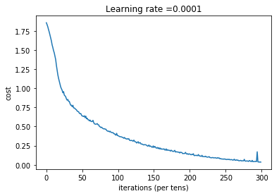
Parameters have been trained!

Train Accuracy: 0.999074

Test Accuracy: 0.725

2.7 - Test with your own image

# import scipy
# from PIL import Image
# from scipy import ndimage
import imageio
from skimage.transform import resize
## START CODE HERE ## (PUT YOUR IMAGE NAME)
my_image = "thumbs_up.jpg"
## END CODE HERE ##
# We preprocess your image to fit your algorithm.
fname = "images/" + my_image
# image = np.array(ndimage.imread(fname, flatten=False))
# my_image = scipy.misc.imresize(image, size=(64,64)).reshape((1, 64*64*3)).T
image = np.array(imageio.imread(fname))                   # 读入图片为矩阵, 这里用原版本的会出错，scipy的那个函数被删了
# print(image.shape)
# 转置图片为 (num_px*num_px*3, 1)向量
my_image = resize(image, output_shape=(64, 64)).reshape((1, 64 * 64 * 3)).T
# print(my_image)
my_image_prediction = predict(my_image, parameters)
plt.imshow(image)
print("Your algorithm predicts: y = " + str(np.squeeze(my_image_prediction)))