论文翻译——Recursive Deep Models for Semantic Compositionality Over a Sentiment Treebank

Abstract

Semantic word spaces have been very useful but cannot express the meaning of longer phrases in a principled way.

语义词空间是非常有用的，但它不能有原则地表达较长短语的意义。

Further progress towards understanding compositionality in tasks such as sentiment detection requires richer supervised training and evaluation resources and more powerful models of composition.

要想在情感检测等任务中进一步理解构成，需要更丰富的监督训练和评估资源，以及更强大的构成模型。

To remedy this, we introduce a Sentiment Treebank.

为了解决这个问题，我们引入了一个情绪树库。

It includes fine grained sentiment labels for 215,154 phrases in the parse trees of 11,855 sentences and presents new challenges for sentiment compositionality.

它为11855个句子的解析树中的215154个短语提供了细粒度的情感标签，并为情感构成提出了新的挑战。

To address them, we introduce the Recursive Neural Tensor Network.

为了解决这个问题，我们引入了递归神经张量网络。

When trained on the new treebank, this model outperforms all previous methods on several metrics.

当在新的树桩上进行训练时，该模型在几个指标上优于以前的所有方法。

It pushes the state of the art in single sentence positive/negative classification from 80% up to 85.4%.

它将单一句子的积极/消极分类从80%提升到85.4%。

The accuracy of predicting fine-grained sentiment labels for all phrases reaches 80.7%, an improvement of 9.7% over bag of features baselines.

预测所有短语的细粒度情绪标签的准确性达到80.7%，比功能包基线提高了9.7%。

Lastly, it is the only model that can accurately capture the effects of negation and its scope at various tree levels for both positive and negative phrases.

最后，它是唯一能够准确捕捉否定效果及其在不同树层次上的范围的模型。

1 Introduction

Semantic vector spaces for single words have been widely used as features (Turney and Pantel, 2010).

单个单词的语义向量空间被广泛用作特征(Turney和Pantel, 2010)。

Because they cannot capture the meaning of longer phrases properly, compositionality in semantic vector spaces has recently received a lot of attention (Mitchell and Lapata, 2010; Socher et al., 2010; Zanzotto et al., 2010; Yessenalina and Cardie, 2011; Socher et al., 2012; Grefenstette et al., 2013).

由于不能正确地捕捉较长短语的含义，语义向量空间中的组合性最近受到了很多关注(Mitchell和Lapata, 2010;Socher等人，2010;Zanzotto等人，2010;Yessenalina和Cardie, 2011年;Socher等人，2012;(Grefenstette et al.， 2013)。

However, progress is held back by the current lack of large and labeled compositionality resources and models to accurately capture the underlying phenomena presented in such data.

然而，由于目前缺乏大型和标记的可组合性资源和模型来准确地捕获这些数据中呈现的潜在现象，这一进展受到了阻碍。

To address this need, we introduce the Stanford Sentiment Treebank and a powerful Recursive Neural Tensor Network that can accurately predict the compositional semantic effects present in this new corpus.

为了满足这一需求，我们引入了斯坦福情感树库和一个强大的递归神经张量网络，它可以准确地预测这一新语料库中出现的成分语义效应。

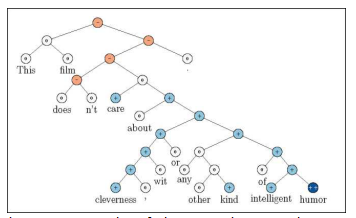
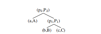
Figure 1: Example of the Recursive Neural Tensor Network accurately predicting 5 sentiment classes, very negative to very positive (- 0, +, + +), at every node of a parse tree and capturing the negation and its scope in this sentence.

图1:递归神经张量网络的例子，准确地预测了5个情绪类，从非常负面到非常正面(- 0，+，+ +)，在解析树的每个节点，捕捉否定和它在这句话中的范围。

The Stanford Sentiment Treebank is the first corpus with fully labeled parse trees that allows for a complete analysis of the compositional effects of sentiment in language.

斯坦福情绪树库是第一个拥有完整标记的解析树的语料库，它允许对语言中情绪的组成影响进行完整的分析。

The corpus is based on the dataset introduced by Pang and Lee (2005) and consists of 11,855 single sentences extracted from movie reviews.

语料库基于庞和李(2005)介绍的数据集，由11,855个从电影评论中提取的单句组成。

It was parsed with the Stanford parser (Klein and Manning, 2003) and includes a total of 215,154 unique phrases from those parse trees, each annotated by 3 human judges.

它是由斯坦福解析器解析的(Klein和Manning, 2003年)，包含了来自这些解析树的总共215,154个独特的短语，每个短语都由3名人类裁判注释。

This new dataset allows us to analyze the intricacies of sentiment and to capture complex linguistic phenomena.

这个新的数据集让我们能够分析情感的复杂性，并捕捉复杂的语言现象。

Fig. 1 shows one of the many examples with clear compositional structure.

图1显示了许多具有清晰的组成结构的例子之一。

The granularity and size of this dataset will enable the community to train compositional models that are based on supervised and structured machine learning techniques.

该数据集的粒度和大小将使社区能够培训基于监督和结构化机器学习技术的组合模型。

While there are several datasets with document and chunk labels available, there is a need to better capture sentiment from short comments, such as Twitter data, which provide less overall signal per document.

虽然有几个带有文档和区块标签的数据集可用，但需要更好地从简短的评论中捕捉情绪，比如Twitter数据，

In order to capture the compositional effects with higher accuracy, we propose a new model called the Recursive Neural Tensor Network (RNTN). Recursive Neural Tensor Networks take as input phrases of any length.

为了获得更准确的成分效应，提出了递归神经张量网络模型。递归神经张量网络作为任意长度的输入短语。

They represent a phrase through word vectors and a parse tree and then compute vectors for higher nodes in the tree using the same tensor-based composition function.

它们通过单词向量和解析树表示短语，然后使用相同的基于时态的组合函数计算树中更高节点的向量。

We compare to several supervised, compositional models such as standard recursive neural networks (RNN) (Socher et al., 2011b), matrix-vector RNNs (Socher et al., 2012), and baselines such as neural networks that ignore word order, Naive Bayes (NB), bi-gram NB and SVM.

我们比较了几种监督的复合模型，如标准递归神经网络(Socher et al.， 2011b)、矩阵向量RNNs (Socher et al.， 2012)，以及基线，如忽略词序的神经网络、朴素贝叶斯(Naive Bayes, NB)、bi-gram NB和SVM。

All models get a significant boost when trained with the new dataset but the RNTN obtains the highest performance with 80.7% accuracy when predicting finegrained sentiment for all nodes.

当使用新数据集进行训练时，所有模型都得到了显著的提升，但是RNTN在预测所有节点的细粒度情绪时获得了最高的性能(80.7%的准确率)。

Lastly, we use a test set of positive and negative sentences and their respective negations to show that, unlike bag of words models, the RNTN accurately captures the sentiment change and scope of negation.

最后，我们使用了一组肯定句和否定句以及它们各自的否定形式来证明，与词汇袋模型不同，RNTN准确地捕捉了情绪变化和否定的范围。

RNTNs also learn that sentiment of phrases following the contrastive conjunction ‘but' dominates.

RNTNs还了解到，短语在对比连接词but之后的感情占主导地位。

The complete training and testing code, a live demo and the Stanford Sentiment Treebank dataset are available at http://nlp.stanford.edu/ sentiment.

完整的训练和测试代码、现场演示和斯坦福情感数据库可以在http://nlp.stanford.edu/ Sentiment上找到。

2 Related Work

This work is connected to five different areas of NLP research, each with their own large amount of related work to which we cannot do full justice given space constraints.

这项工作与5个不同的NLP研究领域相关，每个领域都有大量的相关工作，但由于空间限制，我们无法完全公正地对待这些工作。

Semantic Vector Spaces. The dominant approach in semantic vector spaces uses distributional similarities of single words.

语义向量空间。语义向量空间的主要方法是利用单个词的分布相似性。

Often, co-occurrence statistics of a word and its context are used to describe each word (Turney and Pantel, 2010; Baroni and Lenci, 2010), such as tf-idf.

通常，一个单词及其上下文的共现统计数据被用来描述每个单词(Turney和Pantel, 2010; Baroni和Lenci, 2010)，例如tf-idf。

Variants of this idea use more complex frequencies such as how often a word appears in a certain syntactic context (Pado and Lapata, 2007; Erk and Pad6, 2008).

这种想法的变体使用更复杂的频率，如一个词在特定的句法环境中出现的频率(Pado和Lapata, 2007;Erk和Pad6, 2008)。

However, distributional vectors often do not properly capture the differences in antonyms since those often have similar contexts.

然而，分布向量往往不能很好地捕捉反义词之间的差异，因为它们通常具有相似的上下文。

One possibility to remedy this is to use neural word vectors (Bengio et al., 2003).

一种可能的补救方法是使用神经词向量(Bengio et al., 2003)。

These vectors can be trained in an unsupervised fashion to capture distributional similarities (Collobert and Weston, 2008; Huang et al., 2012) but then also be fine-tuned and trained to specific tasks such as sentiment detection (Socher et al., 2011b).

这些向量可以在无监督的方式下训练，以捕获分布相似性(Collobert和Weston, 2008;(Huang et al.，2012)，但也会针对特定的任务进行微调和培训，如情绪检测(Socher et al.，2011b)。

The models in this paper can use purely supervised word representations learned entirely on the new corpus.

本文的模型完全可以使用在新语料库上学习到的纯监督词表示。

Compositionality in Vector Spaces. Most of the compositionality algorithms and related datasets capture two word compositions.

向量空间的合成性。大多数的合成算法和相关的数据集捕获两个词的合成。

Mitchell and La- pata (2010) use e.g. two-word phrases and analyze similarities computed by vector addition, multiplication and others.

Mitchell和La- pata(2010)使用例如两个单词的短语，并分析由向量加法、乘法等计算出来的相似性。

Some related models such as holographic reduced representations (Plate, 1995), quantum logic (Widdows, 2008), discrete-continuous models (Clark and Pulman, 2007) and the recent compositional matrix space model (Rudolph and Giesbrecht, 2010) have not been experimentally validated on larger corpora.

一些相关的模型如全息简化表示(Plate, 1995)、量子逻辑(Widdows, 2008)、离散-连续模型(Clark and Pulman, 2007)和最近的合成矩阵空间模型(Rudolph and Giesbrecht, 2010)还没有在更大的语料库上进行实验验证。

Yessenalina and Cardie (2011) compute matrix representations for longer phrases and define composition as matrix multiplication, and also evaluate on sentiment.

Yessenalina和Cardie(2011)计算较长短语的矩阵表示，并将组合定义为矩阵乘法，同时根据情感进行评估。

Grefen- stette and Sadrzadeh (2011) analyze subject-verbobject triplets and find a matrix-based categorical model to correlate well with human judgments.

Grefen- stette和Sadrzadeh(2011)分析了主语-动词-宾语三胞胎，并发现了一个基于矩阵的分类模型，该模型与人类的判断密切相关。

We compare to the recent line of work on supervised compositional models. In particular we will describe and experimentally

我们比较了最近关于监督合成模型的工作。特别地，我们将描述和实验比较我们的新RNTN模型与递归神经网络(RNN) (Socher et al.，2011b)和矩阵向量RNNs (Socher et al.， 2012)，这两者都已应用于语料包。

Logical Form. A related field that tackles compositionality from a very different angle is that of trying to map sentences to logical form (Zettlemoyer and Collins, 2005).

逻辑形式。从一个非常不同的角度处理构成的相关领域是试图将句子映射成逻辑形式(Zettlemoyer和Collins, 2005)。

While these models are highly interesting and work well in closed domains and on discrete sets, they could only capture sentiment distributions using separate mechanisms beyond the currently used logical forms.

虽然这些模型非常有趣，而且在封闭域和离散集上都能很好地工作，但它们只能使用当前使用的逻辑形式之外的单独机制来捕获情绪分布。

Deep Learning. Apart from the above mentioned work on RNNs, several compositionality ideas related to neural networks have been discussed by Bot- tou (2011) and Hinton (1990) and Arstmodels such as Recursive Auto-associative memories been experimented with by Pollack (1990).

深度学习。除了上述关于RNNs的工作外，Bot- tou(2011)和Hinton(1990)还讨论了几个与神经网络相关的合成思想，Pollack(1990)还对递归自联想记忆等arstmodel进行了实验。

The idea to relate nh by a tensor have been proposed for relation classification (Sutskever et al., 2009; Jenatton et al., 2012), extending Restricted Boltzmann machines (Ranzato and Hinton, 2010) and as a special layer for speech recognition (Yu et al., 2012).

通过张量将nh联系起来的思想已经被提出用于关系分类(Sutskever et al.，2009; (Jenatton et al.， 2012)，扩展受限玻尔兹曼机(Ranzato and Hinton, 2010)，作为语音识别的特殊层(Yu et al.， 2012)。

Sentiment Analysis. Apart from the above mentioned work, most approaches in sentiment analysis use bag of words representations (Pang and Lee, 2008).

情绪分析。除了上述工作外，情感分析的方法大多采用袋式的词汇表征(Pang和Lee，2008)。

eviews in more detail by analyzing the sentiment of multiple aspects of restaurants, such as food or atmosphere.

通过分析餐厅的食物或氛围等多个方面的情感进行更详细的评论)。

Several works have explored sentiment compositionality through careful engineering of features or polarity shifting rules on syntactic structures (Polanyi and Zaenen, 2006; Moilanen and Pulman, 2007; Rentoumi etal., 2010; Nakagawa etal., 2010).

有几部作品通过仔细研究句法结构的特征或极性转换规则来探索情感构成(Polanyi和Zaenen, 2006;Moilanen和Pulman, 2007;Rentoumi，2010;Nakagawa等等。,2010)。

3 Stanford Sentiment Treebank

Bag of words classifiers can work well in longer documents by relying on a few words with strong sentiment like "awesome5 or "exhilarating?

词袋分类器可以很好地工作在较长的文件依靠几个词与强烈的感情，如“awesome5 or”振奋?”

However, sentiment accuracies even for binary posi- tive/negative classification for single sentences has not exceeded 80% for several years.

然而，即使是对单个句子进行二分正误分类，多年来其情感正确率也没有超过80%。

For the more difficult multiclass case including a neutral class, accuracy is often below 60% for short messages on Twitter (Wang et al., 2012).

对于包含中性类的更困难的多类情况，Twitter上的短消息的准确性通常低于60% (Wang et al.，2012)。

From a linguistic or cognitive standpoint, ignoring word order in the treatment of a semantic task is not plausible, and, as we will show, it cannot accurately classify hard examples of negation.

从语言学或认知的角度来看，在处理语义任务时忽略语序是不合理的，而且，正如我们将展示的，它不能准确地分类否定的硬例子。

Correctly predicting these hard cases is necessary to further improve performance.

正确地预测这些困难情况对于进一步提高性能是必要的。

In this section we will introduce and provide some analyses for the new Sentiment Treebank which includes labels for every syntactically plausible phrase in thousands of sentences, allowing us to train and evaluate compositional models.

在本节中，我们将介绍并提供一些新的情感树库的分析，其中包括标签的每一个看似合理的短语在成千上万的句子，让我们训练和评估组成模型。

We consider the corpus of movie review excerpts from the rottentomatoes. com website originally collected and published by Pang and Lee (2005).

我们考虑了来自rottentom.com网站的电影评论选段，它们最初是由Pang和Lee收集并发表的(2005)。

The original dataset includes 10,662 sentences, half of which were considered positive and lh a longer movie review and reflects the writer's overall intention for this review.

原始数据集包括10662个句子，其中一半被认为是积极的，lh是一个较长的电影评论，反映了作者的总体意图。

The normalized, lowercased text is first used to recover, from the original website, the text with capitalization. Remaining HTML tags and sentences that are not in English are deleted.

规范化、小写的文本首先用于从原始网站恢复大写的文本。其余非英语的HTML标记和句子将被删除。

The Stanford Parser (Klein and Manning, 2003) is used to parses all 10662 sentences.

斯坦福解析器(Klein和Manning, 2003)用于解析所有10,662个句子。

In approximately 1,100 cases it splits the snippet into multiple sentences.

在大约1100个案例中，它将代码片段分成多个句子。

We then used Amazon Mechanical Turk to label the resulting 215,154 phrases.

然后我们使用Amazon Mechanical Turk来标记产生的215,154个短语。

Fig. 3 shows the interface annotators saw.

图3显示了接口注释器saw。

The slider has 25 different values and is initially set to neutral.

滑块有25个不同的值，最初设置为中性。

The phrases in each hit are randomly sampled from the set of all phrases in order to prevent labels being influenced by what follows.

每个命中的短语都是从所有短语中随机抽取的，以防止标签受到以下内容的影响。

For more details on the dataset collection, see supplementary material.

有关数据集收集的更多信息，请参见补充资料。

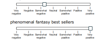
Figure 3: The labeling interface. Random phrases were shown and annotators had a slider for selecting the sentiment and its degree.

图3:标签界面。随机的短语被显示，注释者有一个滑动条来选择情绪和它的程度。

Fig. 2 shows the normalized label distributions at each n-gram length.

图2为各n-gram长度的归一化标签分布。

Starting at length 20, the majority are full sentences.

从20开始，大部分是完整的句子。

One of the findings from labeling sentences based on reader perception is that many of them could be considered neutral.

根据读者的感知给句子贴上标签，其中一个发现是，很多句子可以被认为是中性的。

We also notice that stronger sentiment often builds up in longer phrases and the majority of the shorter phrases are neutral.

我们还注意到，更强烈的情绪往往建立在较长的短语和大多数较短的短语是中性的。

Another observation is that most annotators moved the slider to one of the five positions: negative, somewhat negative, neutral, positive or somewhat positive.

另一个观察结果是，大多数注释器将滑块移动到五个位置之一: 负的、有点负的、中性的、正的或有点正的。

The extreme values were rarely used and the slider was not often left in between the ticks.

极值很少被使用，滑块也不经常被放在刻度之间。

Hence, even a 5-class classification into these categories captures the main variability of the labels.

因此，即使对这些类别进行5类分类，也能捕捉到标签的主要可变性。

We will name this fine-grained sentiment classification and our main experiment will be to recover these five labels for phrases of all lengths.

我们将命名这种细粒度的情感分类，我们的主要实验将是为所有长度的短语恢复这五个标签。

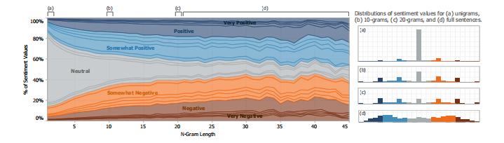
Figure 2: Normalized histogram of sentiment annotations at each n-gram length.

图2:每个n-gram长度的情绪注释的归一化直方图。

Many shorter n-grams are neutral; longer phrases are well distributed.

许多短的n-gram是中性的;较长的短语分布得很好。

Few annotators used slider positions between ticks or the extreme values.

很少有注释器使用刻度之间的滑块位置或极值。

Hence the two strongest labels and intermediate tick positions are merged into 5 classes.

因此，两个最强的标签和中间的蜱位置合并成5类。

4 Recursive Neural Models

The models in this section compute compositional vector representations for phrases of variable length and syntactic type.

本节中的模型计算可变长度和句法类型短语的组成向量表示。

These representations will then be used as features to classify each phrase.

然后这些表示将被用作对每个短语进行分类的特征。

Fig. 4 displays this approach.

图4显示了这种方法。

When an n-gram is given to the compositional models, it is parsed into a binary tree and each leaf node, corresponding to a word, is represented as a vector.

当一个n-gram被赋予组合模型时，它被解析成一个二叉树，每个叶节点对应一个单词，被表示为一个向量。

Recursive neural models will then compute parent vectors in a bottom up fashion using different types of compositionality functions g.

递归神经模型将使用不同类型的合成函数g以自底向上的方式计算父向量。

The parent vectors are again given as features to a classifier. For ease of exposition, we will use the tri-gram in this figure to explain all models.

父向量再次作为特征提供给分类器。为了便于说明，我们将使用图中的三元图来解释所有模型。

We first describe the operations that the below recursive neural models have in common: word vector representations and classification.

我们首先描述以下递归神经模型的共同操作:字向量表示和分类。

This is followed by descriptions of two previous RNN models and our RNTN.

接下来是对前面两个RNN模型和我们的RNTN的描述。

Each word is represented as a d-dimensional vector.

每个单词都表示为d维向量。

We initialize all word vectors by randomly sampling each value from a uniform distribution: W(—r, r), where r = 0.0001.

我们通过从均匀分布中随机抽样每个值来初始化所有的字向量:W(-r, r)，其中r = 0.0001。

All the word vectors are stacked in the word embedding matrix L , where V is the size of the vocabulary.

所有的词向量都堆叠在词嵌入矩阵L中，其中V为词汇量的大小。

Initially the word vectors will be random but the L matrix is seen as a parameter that is trained jointly with the compositionality models.

一开始，词向量是随机的，但是L矩阵被看作是一个与合成模型联合训练的参数。

We can use the word vectors immediately as parameters to optimize and as feature inputs to a soft max classifier.

我们可以直接使用向量作为参数进行优化，并将其作为软最大分类器的特征输入。

For classification into five classes, we compute the posterior probability over labels given the word vector via:

为了将其分为5类，我们通过以下方法计算给定向量的标签的后验概率:

where Ws is the sentiment classification matrix.

其中Ws为情感分类矩阵。

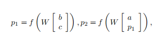
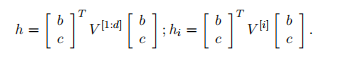
For the given tri-gram, this is repeated for vectors b and c.

对于给定的三元组，这对于向量b和c是重复的。

The main task of and difference between the models will be to compute the hidden vectors pi in a bottom up fashion.

模型之间的主要任务和区别是用自底向上的方式计算隐藏向量pi。

Figure 4: Approach of Recursive Neural Network models for sentiment: Compute parent vectors in a bottom up fashion using a compositionality function g and use node vectors as features for a classififier at that node.

图4:情绪递归神经网络模型方法:使用合成函数g以自底向上的方式计算父向量，并使用节点向量作为该节点上分类器的特征。

This function varies for the different models.

这个函数因不同的模型而异。

4.1 RNN: Recursive Neural Network

The simplest member of this family of neural network models is the standard recursive neural network (Goller and Kiichler, 1996; Socher et al., 2011a).

这个神经网络模型家族中最简单的成员是标准的递归神经网络(Goller and Kiichler, 1996;Socher等，2011a)。

First, it is determined which parent already has all its children computed.

首先，确定哪个父节点已经计算了它的所有子节点。

In the above tree example, pi has its two children's vectors since both are words.

在上面的树的例子中，pi有两个子向量，因为它们都是单词。

RNNs use the following equations to compute the parent vectors:

RNNs使用以下方程来计算父向量:

where f = tanh is a standard element-wise nonlinearity, W is the main parameter to learn and we omit the bias for simplicity.

其中f = tanh是标准的元素非线性，W是需要学习的主要参数，为了简单起见我们省略了偏差。

The bias can be added as an extra column to W if an additional 1 is added to the concatenation of the input vectors.

如果在输入向量的连接中添加额外的1，则可以将偏差作为额外的列添加到W中。

The parent vectors must be of the same dimensionality to be recursively compatible and be used as input to the next composition.

父向量必须具有相同的维数，以便递归兼容，并用作下一个组合的输入。

Each parent vector pi, is given to the same soft max classifier of Eq. 1 to compute its label probabilities.

每一个父向量pi，都被给予相同的软最大分类器Eq. 1来计算它的标签概率。

This model uses the same compositionality function as the recursive autoencoder (Socher et al., 2011b) and recursive auto-associate memories (Pollack, 1990).

该模型使用与递归自编码器(Socher et al.，2011b)和递归自联想记忆(Pollack, 1990)相同的合成功能。

The only difference to the former model is that we fix the tree structures and ignore the reconstruction loss.

与前一种模型的唯一区别是，我们修正了树结构，忽略了重建损失。

In initial experiments, we found that with the additional amount of training data, the reconstruction loss at each node is not necessary to obtain high performance.

在初始实验中，我们发现在训练数据量增加的情况下，每个节点的重构损失并不是获得高性能所必须的。

4.2 MV-RNN: Matrix-Vector RNN

The MV-RNN is linguistically motivated in that most of the parameters are associated with words and each composition function that computes vectors for longer phrases depends on the actual words being combined.

MV-RNN在语言学上是有动机的，因为大多数参数都与单词相关，每个计算长短语向量的复合函数都依赖于实际组合的单词。

The main idea of the MV-RNN (Socher et al., 2012) is to represent every word and longer phrase in a parse tree as both a vector and a matrix.

MV-RNN (Socher et al.，2012)的主要思想是将解析树中的每个单词和更长的短语同时表示为向量和矩阵。

When two constituents are combined the matrix of one is multiplied with the vector of the other and vice versa.

当两个成分结合时，一个的矩阵与另一个的向量相乘，反之亦然。

Hence, the compositional function is parameterized by the words that participate in it.

因此，组合函数是由参与其中的单词参数化的。

Each word's matrix is initialized as a d x d identity matrix, plus a small amount of Gaussian noise.

每个单词的矩阵初始化为一个dxd单位矩阵，加上少量的高斯噪声。

Similar to the random word vectors, the parameters of these matrices will be trained to minimize the classification error at each node.

与随机字向量相似，对这些矩阵的参数进行训练，使每个节点的分类误差最小。

For this model, each n-gram is represented as a list of (vector,matrix) pairs, together with the parse tree.

对于这个模型，每个n-gram都表示为(向量、矩阵)对的列表，以及解析树。

For the tree with (vector,matrix) nodes:

对于有(向量，矩阵)节点的树:

the MV-RNN computes the first parent vector and its matrix via two equations:

MV-RNN通过两个方程计算第一个父向量及其矩阵:

where Wm and the result is again ad x d matrix.

其中Wm的结果仍然是adxd矩阵。

Similarly, the second parent node is computed using the previously computed (vector,matrix) pair (pi, Pi) as well as (a, A).

类似地，第二个父节点使用之前计算的(向量、矩阵)对(pi, pi)和(a, a)进行计算。

The vectors are used for classifying each phrase using the same softmax classifier as in Eq. 1.

使用与公式1中相同的softmax分类器对每个短语进行分类。

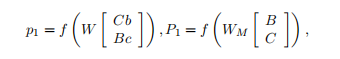
4.3 RNTN:Recursive Neural Tensor Network

One problem with the MV-RNN is that the number of parameters becomes very large and depends on the size of the vocabulary.

MV-RNN的一个问题是参数的数量变得非常大，这取决于词汇表的大小。

It would be cognitively more plausible if there was a single powerful composition function with a fixed number of parameters.

如果只有一个具有固定数量参数的强大复合函数，那么在认知上就更有可能。

The standard RNN is a good candidate for such a function.

标准的RNN是这样一个函数的一个很好的候选。

However, in the standard RNN, the input vectors only implicitly interact through the nonlinearity (squashing) function.

然而，在标准的RNN中，输入向量仅通过非线性(压扁)函数进行隐式交互。

A more direct, possibly multiplicative, interaction would allow the model to have greater interactions between the input vectors.

一个更直接的，可能是乘法的交互将允许模型在输入向量之间有更大的交互。

Motivated by these ideas we ask the question: Can a single, more powerful composition function perform better and compose aggregate meaning from smaller constituents more accurately than many input specific ones?

在这些想法的激励下，我们提出了这样一个问题:一个单独的、功能更强大的复合函数能否比许多特定的输入函数更好地执行并更准确地将更小的成分组合在一起?

In order to answer this question, we propose a new model called the Recursive Neural Tensor Network (RNTN).

为了回答这个问题，我们提出了一个新的模型，称为递归神经张量网络(RNTN)。

The main idea is to use the same, tensor-based composition function for all nodes.

其主要思想是对所有节点使用相同的、基于张应力的组合函数。

Fig. 5 shows a single tensor layer.

图5给出了一个单张量层。

We define the output of a tensor product G via the following vectorized notation and the equivalent but more detailed notation for each slice G:

我们定义了一个张量积G的输出，通过以下矢量化符号和对应的更详细的G切片符号:

where V is the tensor that defines multiple bilinear forms.

其中V是定义多个双线性形式的张量。

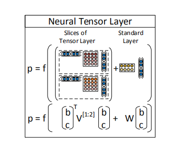
Figure 5: A single layer of the Recursive Neural Tensor Network.

图5:递归神经张量网络的单层图。

Each dashed box represents one of d-many slices and can capture a type of influence a child can have on its parent.

每个虚线框代表一个d-许多片，可以捕获一种类型的影响，一个孩子可以对它的父母。

The RNTN uses this definition for computing pi :

RNTN使用这个定义来计算pi:

where W is as defined in the previous models.

其中W定义在前面的模型中。

The next parent vector P2 in the tri-gram will be computed with the same weights:

三元图中的下一个父向量P2将使用相同的权重计算:

The main advantage over the previous RNN model, which is a special case of the RNTN when V is set to 0, is that the tensor can directly relate input vectors.

与以前的RNN模型相比，它的主要优点是张量可以直接关联输入向量，而以前的模型是当V被设为0时RNTN的一个特例。

Intuitively, we can interpret each slice of the tensor as capturing a specific type of composition.

直观地说，我们可以把张量的每一部分解释为捕捉一种特定类型的成分。

An alternative to RNTNs would be to make the compositional function more powerful by adding a second neural network layer.

RNTNs的另一种替代方法是通过添加第二个神经网络层来增强复合功能。

However, initial experiments showed that it is hard to optimize this model and vector interactions are still more implicit than in the RNTN.

然而，初始实验表明，该模型难以优化，向量间的相互作用仍比RNTN更隐式。

4.4 Tensor Backprop through Structure

We describe in this section how to train the RNTN model.

我们将在本节中描述如何训练RNTN模型。

As mentioned above, each node has a softmax classifier trained on its vector representation to predict a given ground truth or target vector *t.

如前所述，每个节点都有一个针对其向量表示的softmax分类器来预测给定的地面真值或目标向量*t。

We assume the target distribution vector at each node has a 0-1 encoding.

我们假设每个节点的目标分布向量都是0-1编码。

If there are C classes, then it has length C and a 1 at the correct label.

如果有C类，那么它在正确的标签处有C和1。

All other entries are 0.

其他所有项都是0。

We want to maximize the probability of the correct prediction, or minimize the cross-entropy error between the predicted distribution R at node iand the target distribution R at that node.

我们想要最大化正确预测的概率，或者最小化预测的分布R在节点i上与目标分布R在节点i上的交叉熵误差。

This is equivalent (up to a constant) to minimizing the KL-divergence between the two distributions.

这与最小化两个分布之间的kl -散度是等价的(至多是一个常数)。

The error as a function of the RNTN parameters (V, W, W_s, L) for a sentence is:

一个句子的错误作为RNTN参数(V, W, W_s, L)的函数为:

The derivative for the weights of the softmax classifier are standard and simply sum up from each node's error.

softmax分类器的权值的导数是标准的，简单地从每个节点的误差求和。

We define to be the vector at node i (in the example trigram, the e R are (a, b, c, p_1, p_2)) We skip the standard derivative for W.

我们定义为节点i处的向量(在例子中，e R是(a, b, c, p_1, p_2))我们跳过了W*的标准导数。

Each node backpropagates its error through to the recursively used weights V, W.

每个节点将其错误反向传播到递归使用的权值V, W。

Let R be the softmax error vector at node i:

设R为节点i处的softmax误差向量:

where is the Hadamard product between he two vectors and f is the element-wise derivative of f which in the standard case of using f = tanh can be computed using only f (x^i).

其中，两个向量之间的Hadamard 积，f是f的元素级导数，在使用f = tanh的标准情况下，可以只使用f (x^i)来计算。

The remaining derivatives can only be computed in a top-down fashion from the top node through the tree and into the leaf nodes.

其余的导数只能以自顶向下的方式计算，从顶部节点开始，经过树，然后进入叶节点。

The full derivative for V and W is the sum of the derivatives at each of the nodes.

V和W的完整导数是每个节点上导数的和。

We define the complete incoming error messages for a node i as R. The top node, in our case p2, only received errors from the top node's softmax.

我们将一个节点i的完整传入错误消息定义为r。顶部节点(在我们的示例中为p2)仅接收来自顶部节点的softmax的错误。

Hence, which we can use to obtain the standard backprop derivative for W (Goller and Kiichler, 1996;Socher et al., 2010).

因此，我们可以用它来得到W的标准支撑物导数(Goller and Kiichler, 1996;Socher等人，2010)。

For the derivative of each slice k = 1,..., d, we get:

对于每一片的导数k = 1，…, d，得到:

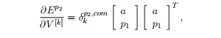
where is just the Afth element of this vector.

其中是这个向量的第n个元素。

Now, we can compute the error message for the two children of p2:

现在，我们可以计算p2的两个子元素的错误信息:

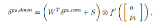
where we define

我们定义

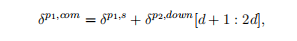
The children of p_2，will then each take half of this vector and add their own soft max error message for the complete R. In particular, we have

然后，p_2的子元素，每个元素将取这个向量的一半，并为整个r添加它们自己的软最大错误消息然后，

where [d+1] indicates that pi is the right child of p2 and hence takes the 2nd half of the error, for the final word vector derivative for a, it will be [1:d].

其中[d+1]表示pi是p2的右子元素，因此取误差的后半部分，对于a的最终向量导数，它将是[1:d]。

The full derivative for slice for this trigram tree then is the sum at each node:

这个三元树的切片的完整导数是每个节点的和:

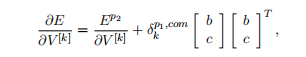
and similarly for W. For this nonconvex optimization we use AdaGrad (Duchi etal., 2011) which converges in less than 3 hours to a local optimum.

对于W也是类似的。对于这种非凸优化，我们使用AdaGrad (Duchi etal.)。在不到3小时内收敛到局部最优。

5 Experiments

We include two types of analyses.

我们包括两种类型的分析。

The first type includes several large quantitative evaluations on the test set. The second type focuses on two linguistic phenomena that are important in sentiment.

第一种类型包括对测试集的几项大型定量评估。第二种类型侧重于两种对情绪很重要的语言现象。

For all models, we use the dev set and crossvalidate over regularization of the weights, word vector size as well as learning rate and minibatch size for AdaGrad.

For models, 我们 使用 dev 设置 和 crossvalidate 正规化 weights, 词 向量 大小 以及 学习 速率 和 minibatch AdaGrad. 大小

Optimal performance for all models was achieved at word vector sizes between 25 and 35 dimensions and batch sizes between 20 and 30.

所有模型的最佳性能都是在25到35维的字向量大小和20到30维的批处理大小之间实现的。

Performance decreased at larger or smaller vector and batch sizes.

性能下降在较大或较小的矢量和批量大小。

This indicates that the RNTN does not outperform the standard RNN due to simply having more parameters.

这表明，RNTN并不优于标准RNN，原因仅仅是参数更多。

The MV-RNN has orders of magnitudes more parameters than any other model due to the word matrices.

由于矩阵的存在，使得MV-RNN的参数比其他任何模型都多几个数量级。

The RNTN would usually achieve its best performance on the dev set after training for 3 - 5 hours.

RNTN通常会在训练3 - 5小时后在开发集上取得最佳表现。

Initial experiments showed that the recursive models worked significantly worse (over 5% drop in accuracy) when no nonlinearity was used.

q初始实验表明，在不使用非线性的情况下，递归模型的性能明下降(精度下降超过5%)。

We use f = tanh in all experiments.

我们在所有的实验中都使用f = tanh。

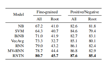
Table 1: Accuracy for fine grained (5-class) and binary predictions at the sentence level (root) and for all nodes.

表1:句子级(根级)和所有节点上细粒度(5级)和二进制预测的准确性。

We compare to commonly used methods that use bag of words features with Naive Bayes and SVMs, as well as Naive Bayes with bag of bigram features.

我们比较了常用的使用朴素贝叶斯和支持向量机的词包特征的方法，以及使用二元特征包的朴素贝叶斯方法。

We abbreviate these with NB, SVM and biNB.

我们用NB, SVM和biNB来简化它们。

We also compare to a model that averages neural word vectors and ignores word order (VecAvg).

我们还比较了一个平均神经词向量和忽略词序(VecAvg)的模型。

The sentences in the treebank were split into a train (8544), dev (1101) and test splits (2210) and these splits are made available with the data release.

“树银行”中的句子被分为火车(8544)、dev(1101)和测试拆分(2210)，这些拆分在数据发布时可用。

We also analyze performance on only positive and negative sentences, ignoring the neutral class.

我们也只分析肯定句和否定句的表现，忽略了中性句。

This filters about 20% of the data with the three sets having 6920/872/1821 sentences.

This 过滤器 大约 20% 的 数据 与 三 组 having 6920/872/1821 sentences.

5.1 Fine-grained Sentiment For All Phrases

The main novel experiment and evaluation metric analyze the accuracy of fine-grained sentiment classification for all phrases.

主要的新颖实验和评价指标分析了细粒度情绪分类的准确性。

Fig. 2 showed that a fine grained classification into 5 classes is a reasonable approximation to capture most of the data variation.

从图2可以看出，将细粒度划分为5个类是捕获大部分数据变化的合理近似方法。

Fig. 6 shows the result on this new corpus.

图6显示了这个新语料库的结果。

The RNTN gets the highest performance, followed by the MV-RNN and RNN.

RNTN的性能最高，其次是MV-RNN和RNN。

The recursive models work very well on shorter phrases, where negation and composition are important, while bag of features baselines perform well only with longer sentences.

递归模型在短句上运行得很好，短句中否定和合成很重要，而大量的特征基线只在长句上运行得很好。

The RNTN accuracy upper bounds other models at most n-gram lengths.

RNTN的精度上限是其他模型在最多n克长度处的上限。

Table 1 (left) shows the overall accuracy numbers for fine grained prediction at all phrase lengths and full sentences.

表1(左)显示了所有短语长度和完整句子的细粒度预测的总体准确率。

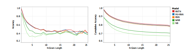
Figure 6: Accuracy curves for fine grained sentiment classification at each n-gram lengths.

图6:每个n克长度的细粒度情绪分类的准确性曲线。

Left: Accuracy separately for each set of n-grams.

左:每组n-grams的准确性分别。

Right: Cumulative accuracy of all < n-grams.

右:所有< n-grams的累积精度。

5.2 Full Sentence Binary Sentiment

This setup is comparable to previous work on the original rotten tomatoes dataset which only used full sentence labels and binary classification of positive/negative.

这个设置与之前在烂番茄网站的原始数据集上仅使用完整句子标签和词性/否定的二元分类的工作类似。

Hence, these experiments show the improvement even baseline methods can achieve with the sentiment treebank.

因此，这些实验表明，改进甚至基线方法可以实现与情绪树银行。

Table 1 shows results of this binary classification for both all phrases and for only full sentences.

表1显示了所有短语和完整句子的二分类结果。

The previous state of the art was below 80% (Socher et al., 2012).

以前的技术水平低于80% (Socher et al.， 2012)。

With the coarse bag of words annotation for training, many of the more complex phenomena could not be captured, even by more powerful models.

用粗糙的单词注释训练，许多更复杂的现象不能被捕获，即使是更强大的模型。

The combination of the new sentiment treebank and the RNTN pushes the state of the art on short phrases up to 85.4%.

“新情绪树银行”和“RNTN”的结合使得最新潮的短短语达到了85.4%。

5.3 Model Analysis: Contrastive Conjunction

In this section, we use a subset of the test set which includes only sentences with an ‘X but Y" structure:

在本节中,我们使用测试集的一个子集,包括句子的X但Y”结构:

A phrase X being followed by but which is followed by a phrase Y. The conjunction is interpreted as an argument for the second conjunct, with the first functioning concessively (Lakoff, 1971;Blakemore, 1989;Merin, 1999).Fig. 7 contains an example.

一个短语X 但紧随其后紧随其后的是一个短语Y的结合是第二次结合的解释作为参数,与第一个让步地运作(Lakoff, 1971;布莱克莫尔,1989;Merin, 1999)。图7包含一个示例。

We analyze a strict setting, where X and Y are phrases of different sentiment (including neutral).

我们分析了一个严格的设置，其中X和Y是不同情绪的短语(包括中性的)。

The example is counted as correct, if the classifications for both phrases X and Y are correct.

如果短语X和*Y的分类都是正确的，那么这个例子就被认为是正确的。

Furthermore, the lowest node that dominates both of the word but and the node that spans Y also have to have the same correct sentiment.

此外，同时控制but和跨越*Y的节点的最低节点也必须具有相同的正确情绪。

For the resulting 131 cases, the RNTN obtains an accuracy of 41% compared to MV-RNN (37), RNN (36) and biNB (27).

在得到的131个病例中，RNTN与MV-RNN(37)、RNN(36)和biNB(27)相比，其准确率为41%。

5.4 Model Analysis: High Level Negation

We investigate two types of negation. For each type, we use a separate dataset for evaluation.

我们研究了两种类型的否定。对于每种类型，我们使用单独的数据集进行评估。

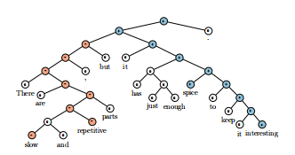
Figure 7: Example of correct prediction for contrastive conjunction X but Y.

图7:对比连词X与Y正确预测的例子。

Set 1: Negating Positive Sentences. The first set contains positive sentences and their negation.

设置1:否定肯定句。第一组包含肯定句和否定句。

In this set, the negation changes the overall sentiment of a sentence from positive to negative.

在这组句子中，否定句把句子的整体情绪由肯定变为否定。

Hence, we compute accuracy in terms of correct sentiment reversal from positive to negative.

因此，我们根据从正面到负面的正确情绪逆转来计算准确性。

Fig. 9 shows two examples of positive negation the RNTN correctly classified, even if negation is less obvious in the case of 'least'.

图9给出了RNTN正确分类的两个肯定否定的例子，即使否定在“最小”的情况下不那么明显。

Table 2 (left) gives the accuracies over 21 positive sentences and their negation for all models.

表2(左)给出了所有模型中超过21个肯定句和否定句的准确性。

The RNTN has the highest reversal accuracy, showing its ability to structurally learn negation of positive sentences.

RNTN具有最高的反转精度，显示出它在结构上学习否定肯定句的能力。

But what if the model simply makes phrases very negative when negation is in the sentence?

但是，如果当否定句出现在句子中时，该模型只是让短语变得非常否定呢?

The next experiments show that the model captures more than such a simplistic negation rule.

接下来的实验表明，该模型捕获的不仅仅是这样一个简单的否定规则。

Set 2: Negating Negative Sentences. The second set contains negative sentences and their negation.

设置2:否定否定句。第二组包含否定句和否定句。

When negative sentences are negated, the seniment treebank shows that overall sentiment should become less negative, but not necessarily positive.

当否定句被否定时，实验数据库显示整体情绪应该变得不那么消极，但不一定是积极的。

For instance, "The movie was terrible, is negative but the "The movie was not terrible, says only that it was less bad than a terrible one, not that it was good (Horn, 1989;

例如，“这部电影很糟糕，是消极的，但”这部电影并不糟糕，只是说它比糟糕的电影差，不是说它好(霍恩，1989;Israel, 2001).以色列,2001)。

Hence, we evaluate accuracy in terms of how often each model was able to increase non-negative activation in the sentiment of the sentence.

因此，我们根据每个模型增加句子非负性激活的频率来评估准确性。

Table 2 (right) shows the accuracy.

表2(右)显示了准确性。

In over 81% of cases, the RNTN correctly increases the positive activations.

在81%以上的病例中，RNTN正确地增加了阳性激活。

Fig. 9 (bottom right) shows a typical case in which sentiment was made more positive by switching the main class from negative to neutral even though both not and dull were negative.

图9(右下角)显示了一个典型的案例，在这个案例中，尽管not和dull都是负面的，但通过将主类从负面转换为中性，情绪变得更加积极。

Fig. 8 shows the changes in activation for both sets.

图8显示了两组的激活变化。

Negative values indicate a decrease in average positive activation (for set 1) and positive values mean an increase in average positive activation (set 2). The RNTN has the largest shifts in the correct directions.

负值表示平均正激活减少(对于集合1)，正值表示平均正激活增加(对于集合2)。RNTN在正确方向上的变化最大。

Figure 9: RNTN prediction of positive and negative (bottom right) sentences and their negation.

图9:RNTN预测肯定句和否定句(右下)和否定句。

Table 2: Accuracy of negation detection. Negated positive is measured as correct sentiment inversions. Negated negative is measured as increases in positive activations.

表2:否定检测的准确性。消极的积极被认为是正确的情绪逆转。负性是指阳性激活量的增加。

Therefore we can conclude that the RNTN is best able to identify the effect of negations upon both positive and negative sentiment sentences.

因此，我们可以得出结论，RNTN最能识别否定词对肯定句和否定句的影响。

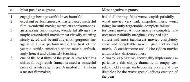
Table 3: Examples of n-grams for which the RNTN predicted the most positive and most negative responses.

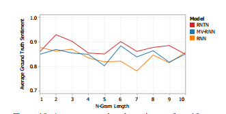
Figure 10: Average ground truth sentiment of top 10 most positive n-grams at various n. The RNTN correctly picks the more negative and positive examples.

5.5 Model Analysis: Most Positive and Negative Phrases

We queried the model for its predictions on what the most positive or negative n-grams are, measured as the highest activation of the most negative and most positive classes. Table 3 shows some phrases from the dev set which the RNTN selected for their strongest sentiment.

Due to lack of space we cannot compare top phrases of the other models but Fig. 10 shows that the RNTN selects more strongly positive phrases at most n-gram lengths compared to other models.

For this and the previous experiment, please find additional examples and descriptions in the supplementary material.

6 Conclusion

We introduced Recursive Neural Tensor Networks and the Stanford Sentiment Treebank.

我们介绍了递归神经张量网络和斯坦福情绪树库。

The combination of new model and data results in a system for single sentence sentiment detection that pushes state of the art by 5.4% for positive/negative sentence classification.

The combination 新 模型 和 数据 的 结果 在 一 个 单一 的 句子 情感 探测 系统 , 将 先进 的 5.4% classification. positive/negative 句子

Apart from this standard setting, the dataset also poses important new challenges and allows for new evaluation metrics.

除了这个标准设置，数据集还提出了重要的新挑战，并允许新的评估指标。

For instance, the RNTN obtains 80.7% accuracy on fine-grained sentiment prediction across all phrases and captures negation of different sentiments and scope more accurately than previous models.

例如，RNTN在对所有短语的细粒度情绪预测上获得80.7%的准确性，并比以前的模型更准确地捕获对不同情绪和范围的否定。

Acknowledgments

We thank Rukmani Ravisundaram and Tayyab Tariq for the first version of the online demo.

我们感谢Rukmani Ravisundaram和Tayyab Tariq提供了第一个在线演示版本。

Richard is partly supported by a Microsoft Research PhD fellowship.

Richard 部分 支持 Microsoft Research PhD fellowship.

The authors gratefully acknowledge the support of the Defense Advanced Research Projects Agency (DARPA) Deep Exploration and Filtering of Text (DEFT) Program under Air Force Research Laboratory (AFRL) prime contract no.

作者非常感谢美国国防部高级研究计划局(DARPA)对美国空军研究实验室(AFRL)主合同。

FA8750-13-2-0040, the DARPA Deep Learning program under contract number FA8650-10-C-7020 and NSF IIS-1159679.

合同编号为FA8650-10-C-7020和NSF ii -1159679。

Any opinions, findings, and conclusions or recommendations expressed in this material are those of the authors and do not necessarily reflect the view of DARPA, AFRL, or the US government.

本材料中表达的任何观点、发现、结论或建议均为作者的观点，并不一定反映DARPA、AFRL或美国政府的观点。

References

M. Baroni and A. Lenci. 2010. Distributional memory: A general framework for corpus-based semantics. Computational Linguistics, 36(4):673-721.

Y. Bengio, R. Ducharme, P. Vincent, and C. Janvin. 2003. A neural probabilistic language model. J. Mach. Learn. Res., 3, March.

D. Blakemore. 1989. Denial and contrast: A relevance theoretic analysis of 'but'. Linguistics and Philosophy, 12:15-37.

L. Bottou. 2011. From machine learning to machine reasoning. CoRR, abs/1102.1808.

S. Clark and S. Pulman. 2007. Combining symbolic and distributional models of meaning. In Proceedings of the AAAI Spring Symposium on Quantum Interaction, pages 52-55.

R. Collobert and J. Weston. 2008. A unified architecture for natural language processing: deep neural networks with multitask learning. In ICML.

J. Duchi, E. Hazan, and Y. Singer. 2011. Adaptive subgradient methods for online learning and stochastic optimization. J MLR, 12, July.

K. Erk and S. Pado. 2008. A structured vector space model for word meaning in context. In EMNLP.

C. Goller and A. Kiichler. 1996. Learning taskdependent distributed representations by backpropaga- tion through structure. In Proceedings of the International Conference on Neural Networks (ICNN-96).

E. Grefenstette and M. Sadrzadeh. 2011. Experimental support for a categorical compositional distributional model of meaning. In EMNLP.

E. Grefenstette, G. Dinu, Y.-Z. Zhang, M. Sadrzadeh, and M. Baroni. 2013. Multi-step regression learning for compositional distributional semantics. In IWCS.

G. E. Hinton. 1990. Mapping part-whole hierarchies into connectionist networks. Artificial Intelligence, 46(12).

L. R. Hom. 1989. A natural history of negation, volume 960. University of Chicago Press Chicago.

E. H. Huang, R. Socher, C. D. Manning, and A. Y. Ng. 2012. Improving Word Representations via Global Context and Multiple Word Prototypes. In ACL.

M. Israel. 2001. Minimizers, maximizers, and the rhetoric of scalar reasoning. Journal of Semantics, 18(4):297-331.

R. Jenatton, N. Le Roux, A. Bordes, and G. Obozinski. 2012. A latent factor model for highly multi-relational data. In NIPS.

D. Klein and C. D. Manning. 2003. Accurate unlexical- ized parsing. In ACL.

R. Lakoff. 1971. IPs, and's, and bufs about conjunction. In Charles J. Fillmore and D. Terence Langendoen, editors, Studies in Linguistic Semantics, pages 114-149. Holt, Rinehart, and Winston, New York.

A. Merin. 1999. Information, relevance, and social decisionmaking: Some principles and results of decision- theoretic semantics. In Lawrence S. Moss, Jonathan Ginzburg, and Maarten de Rijke, editors, Logic, Language, and Information, volume 2. CSLI, Stanford, CA.

J. Mitchell and M. Lapata. 2010. Composition in distributional models of semantics. Cognitive Science, 34(8):1388-1429.

K. Moi质enand S. Pulman,2007. Sentimentcomposition. In In Proceedings of Recent Advances in Natural Language Processing.

T. Nakagawa, K. Inui, and S. Kurohashi. 2010. Dependency tree-based sentiment classification using CRFs with hidden variables. In NAACL, HLT.

S. Pado 弧d M. Lapata, 2007. Dependency-based construction of semantic space models. Computational Linguistics, 33(2):161-199.

B. Pang andL. Lee. 2005. Seeing stars: Exploiting class relationships for sentiment categorization with respect to rating scales. In ACL, pages 115-124.

B. Pang and L. Lee. 2008. Opinion mining and sentiment analysis. Foundations and Trends in Information Retrieval, 2(1-2):1-135.

T. A. Plate. 1995. Holographic reduced representations. IEEE Transactions on Neural Networks, 6(3):623- 641.

L. Polanyi and A. Zaenen. 2006. Contextual valence shifters. In W. Bruce Croft, James Shanahan, Yan Qu, and Janyce Wiebe, editors, Computing Attitude and Affect in Text: Theory and Applications, volume 20 of The Information Retrieval Series, chapter 1.

J. B. Pollack. 1990. Recursive distributed representations. Artificial Intelligence, 46, November.

M. Ranzato and A. Krizhevsky G. E. Hinton. 2010. Factored 3-Way Restricted Boltzmann Machines For Modeling Natural Images. AISTATS.

V. Rentoumi, S. Petrakis, M. Klenner, G. A. Vburos, and V. Karkaletsis. 2010. United we stand: Improving sentiment analysis by joining machine learning and rule based methods. In Proceedings of the Seventh conference on International Language Resources and Evaluation (LREC'10), Valletta, Malta.

S. Rudolph and E. Giesbrecht. 2010. Compositional matrix-space models of language. In ACL.

B. Snyder and R. Barzilay. 2007. Multiple aspect ranking using the Good Grief algorithm. In HLT-NAACL.

R. Socher, C. D. Manning, and A. Y. Ng. 2010. Learning continuous phrase representations and syntactic parsing with recursive neural networks. In Proceedings of the NIPS-2010 Deep Learning and Unsupervised Feature Learning Workshop.