(原)Non-local Neural Networks
转载请注明出处:
https://www.cnblogs.com/darkknightzh/p/12592351.html
论文:
https://arxiv.org/abs/1711.07971
第三方pytorch代码:
https://github.com/AlexHex7/Non-local_pytorch
1. non local操作
该论文定义了通用了non local操作:
${{\mathbf{y}}_{i}}=\frac{1}{C(\mathbf{x})}\sum\limits_{\forall j}{f({{\mathbf{x}}_{i}},{{\mathbf{x}}_{j}})g({{\mathbf{x}}_{j}})}$
其中i为需要计算响应的输出位置的索引,j为所有的位置。x为输入信号(图像,序列,视频等,通常为这些信号的特征),y为个x相同尺寸的输出信号。f为pairwise的函数,f计算当前i和所有j之间的关系,并得到一个标量。一元函数g计算输入信号在位置j的表征。(这段翻译起来怪怪的)。C(x)为归一化系数,用于归一化f和g的结果。
2. non local和其他操作的区别
① non local考虑到了所有的位置j。卷积操作仅考虑了当前位置的一个邻域(如核为3的一维卷积仅考虑了i-1<=j<=i+1);循环操作通常只考虑当前和上一个时间,j=i或j=i-1.
② non local根据不同位置的关系计算响应,fc使用学习到的权重。换言之,fc中,${{\mathbf{x}}_{i}}$和${{\mathbf{x}}_{j}}$之间不是函数关系,而non local中则是函数关系。
③ non local支持输入不同尺寸,并且保持输出和输入相同的尺寸;fc则需要输入和输出均为固定的尺寸,并且丢失了位置关系。
④ non local可以用在网络的早期部分,fc通常用在网络最后。
3. f和g的形式
3.1 g的形式
为简单起见,只考虑g为线性形式,$g({{\mathbf{x}}_{j}})\text{=}{{W}_{g}}{{\mathbf{x}}_{j}}$,${{W}_{g}}$为需要学习的权重向量,在空域可以使用1*1conv实现,在空间时间域(如时间序列的图像)可以通过1*1*1的卷积实现。
3.2 f为gaussian
$f({{\mathbf{x}}_{i}},{{\mathbf{x}}_{j}})\text{=}{{e}^{\mathbf{x}_{i}^{T}{{\mathbf{x}}_{j}}}}$
其中$\mathbf{x}_{i}^{T}{{\mathbf{x}}_{j}}$为点乘,因为点乘在深度学习平台中更易实现(欧式距离也可以)。此时归一化系数$C(\mathbf{x})=\sum\nolimits_{\forall j}{f({{\mathbf{x}}_{i}},{{\mathbf{x}}_{j}})}$
3.3 f为embedded Gaussian
$f({{\mathbf{x}}_{i}},{{\mathbf{x}}_{j}})\text{=}{{e}^{\theta {{({{\mathbf{x}}_{i}})}^{T}}\phi ({{\mathbf{x}}_{j}})}}$
其中$\theta ({{\mathbf{x}}_{i}})\text{=}{{W}_{\theta }}{{\mathbf{x}}_{i}}$,$\phi ({{\mathbf{x}}_{j}})\text{=}{{W}_{\phi }}{{\mathbf{x}}_{j}}$,此时$C(\mathbf{x})=\sum\nolimits_{\forall j}{f({{\mathbf{x}}_{i}},{{\mathbf{x}}_{j}})}$
self attention模块和non local的关系:可以认为self attention为embedded Gaussian的特殊形式,如给定i,$\frac{1}{C(\mathbf{x})}f({{\mathbf{x}}_{i}},{{\mathbf{x}}_{j}})$沿着j维度变成了计算softmax。此时$\mathbf{y}=softmax({{\mathbf{x}}^{T}}W_{\theta }^{T}{{W}_{\phi }}\mathbf{x})g(\mathbf{x})$,即为self attention的形式。
3.4 点乘
f可以定义为点乘的相似度(此处使用embedded的形式):
$f({{\mathbf{x}}_{i}},{{\mathbf{x}}_{j}})\text{=}\theta {{({{\mathbf{x}}_{i}})}^{T}}\phi ({{\mathbf{x}}_{j}})$
此时,归一化系数$C(\mathbf{x})=N$,N为x中所有位置的数量,而不是f的sum,这样可以简化梯度的计算。
点乘和embedded Gaussian的区别是是否使用了作为激活函数的softmax。
3.5 Concatenation
$f({{\mathbf{x}}_{i}},{{\mathbf{x}}_{j}})\text{=ReLU(w}_{f}^{T}[\theta ({{\mathbf{x}}_{i}}),\phi ({{\mathbf{x}}_{j}})]\text{)}$
其中$[\cdot \cdot ]$代表concatenation,即拼接。${{w}_{f}}$为权重向量,用于将拼接后的向量映射到一个标量。$C(\mathbf{x})=N$
4. Non local block
将之前公式的non local操作扩展成non local block,可以嵌入到目前的网络结构中,如下:
${{\mathbf{z}}_{i}}={{W}_{z}}{{\mathbf{y}}_{i}}+{{\mathbf{x}}_{i}}$
其中${{\mathbf{y}}_{i}}=\frac{1}{C(\mathbf{x})}\sum\limits_{\forall j}{f({{\mathbf{x}}_{i}},{{\mathbf{x}}_{j}})g({{\mathbf{x}}_{j}})}$,$+{{\mathbf{x}}_{i}}$代表残差连接。残差连接方便将non local block嵌入到之前与训练的模型中,避免打乱其初始行为(如将${{W}_{z}}$初始化为0)。
non local block如下图所示。3.2,3.3,3.4中的pairwise计算对应于下图中的矩阵乘法。在网络后面的特征图上,pairwise计算量比较小。
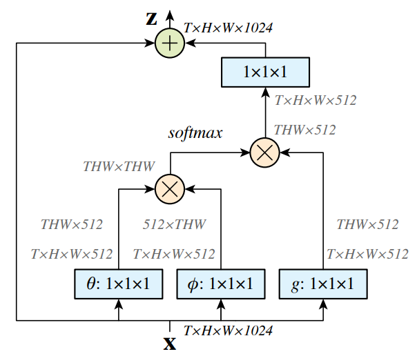
说明:
1. 若为图像,则使用1*1conv,且图中无T;若为视频,则使用1*1*1conv,且图中有T。
2. 图中softmax指对该矩阵每行计算softmax。
5. 降低计算量
5.1 降低x的通道数量
将${{W}_{g}}$,${{W}_{\theta }}$,${{W}_{\phi }}$降低为x的通道数量的一半,可以降低计算量。
5.2 对x下采样。
对x下采样,可以进一步降低计算量。
此时,1中的共识修改为${{\mathbf{y}}_{i}}=\frac{1}{C(\mathbf{\hat{x}})}\sum\limits_{\forall j}{f({{\mathbf{x}}_{i}},{{{\mathbf{\hat{x}}}}_{j}})g({{{\mathbf{\hat{x}}}}_{j}})}$,其中$\mathbf{\hat{x}}$为对x进行下采样后的输入(如pooling)。这种方式可以降低pariwsie计算到原来的1/4,一方面不影响non local的行为,另一方面,使得计算更加稀疏。可以通过在上图中$\phi $和$g$后面加一个max pooling来实现。
6. 代码:
6.1 embedded_gaussian
 class _NonLocalBlockND(nn.Module):

     def __init__(self, in_channels, inter_channels=None, dimension=3, sub_sample=True, bn_layer=True):

         """

         :param in_channels:

         :param inter_channels:

         :param dimension:

         :param sub_sample:

         :param bn_layer:

         """

         super(_NonLocalBlockND, self).__init__()

         assert dimension in [1, 2, 3]

         self.dimension = dimension

         self.sub_sample = sub_sample

         self.in_channels = in_channels

         self.inter_channels = inter_channels

         if self.inter_channels is None:

             self.inter_channels = in_channels // 2

             if self.inter_channels == 0:

                 self.inter_channels = 1

         if dimension == 3:

             conv_nd = nn.Conv3d

             max_pool_layer = nn.MaxPool3d(kernel_size=(1, 2, 2))

             bn = nn.BatchNorm3d

         elif dimension == 2:

             conv_nd = nn.Conv2d

             max_pool_layer = nn.MaxPool2d(kernel_size=(2, 2))

             bn = nn.BatchNorm2d

         else:

             conv_nd = nn.Conv1d

             max_pool_layer = nn.MaxPool1d(kernel_size=(2))

             bn = nn.BatchNorm1d

         self.g = conv_nd(in_channels=self.in_channels, out_channels=self.inter_channels,

                          kernel_size=1, stride=1, padding=0)    # g函数,1*1conv,用于降维

         if bn_layer:

             self.W = nn.Sequential(    # 1*1conv,用于图2中变换到原始维度

                 conv_nd(in_channels=self.inter_channels, out_channels=self.in_channels,

                         kernel_size=1, stride=1, padding=0),

                 bn(self.in_channels)

             )

             nn.init.constant_(self.W[1].weight, 0)

             nn.init.constant_(self.W[1].bias, 0)

         else:

             self.W = conv_nd(in_channels=self.inter_channels, out_channels=self.in_channels,

                              kernel_size=1, stride=1, padding=0)   # 1*1conv,用于图2中变换到原始维度

             nn.init.constant_(self.W.weight, 0)

             nn.init.constant_(self.W.bias, 0)

         self.theta = conv_nd(in_channels=self.in_channels, out_channels=self.inter_channels,

                              kernel_size=1, stride=1, padding=0)   # θ函数,1*1conv,用于降维

         self.phi = conv_nd(in_channels=self.in_channels, out_channels=self.inter_channels,

                            kernel_size=1, stride=1, padding=0)    # φ函数,1*1conv,用于降维

         if sub_sample:

             self.g = nn.Sequential(self.g, max_pool_layer)

             self.phi = nn.Sequential(self.phi, max_pool_layer)

     def forward(self, x, return_nl_map=False):

         """

         :param x: (b, c, t, h, w)

         :param return_nl_map: if True return z, nl_map, else only return z.

         :return:

         """

         # 令x维度B*C*(K):一维时,x为B*C*(K1);二维时,x为B*C*(K1*K2);三维时,x为B*C*(K1*K2*K3)

         batch_size = x.size(0)   # batchsize

         g_x = self.g(x).view(batch_size, self.inter_channels, -1)   # 通过g函数,并reshape,得到B*inter_channels*(K)矩阵

         g_x = g_x.permute(0, 2, 1)   # 得到B*(K)*inter_channels矩阵,和图2中一致

         theta_x = self.theta(x).view(batch_size, self.inter_channels, -1)   # 通过θ函数,并reshape,得到B*inter_channels*(K)矩阵

         theta_x = theta_x.permute(0, 2, 1)   # 得到B*(K)*inter_channels矩阵,和图2中一致

         phi_x = self.phi(x).view(batch_size, self.inter_channels, -1)   # 通过φ函数,并reshape,得到B*inter_channels*(K)矩阵

         f = torch.matmul(theta_x, phi_x)    # 得到B*(K)*(K)矩阵,和图2中一致

         f_div_C = F.softmax(f, dim=-1)      # 通过softmax,对最后一维归一化,得到归一化的特征,即概率,B*(K)*(K)

         y = torch.matmul(f_div_C, g_x)      # 得到B*(K)*inter_channels矩阵,和图2中一致

         y = y.permute(0, 2, 1).contiguous() # 得到B*inter_channels*(K)矩阵,和图2中一致

         y = y.view(batch_size, self.inter_channels, *x.size()[2:])  # 得到B*inter_channels*(K1或K1*K2或K1*K2*K3)矩阵,和图2中一致

         W_y = self.W(y)  # 得到B*C*(K)矩阵,和图2中一致

         z = W_y + x   # 特征图和non local的图相加,得到新的特征图,B*C*(K)

         if return_nl_map:

             return z, f_div_C   # 返回结果及归一化的特征

         return z

 class NONLocalBlock1D(_NonLocalBlockND):

     def __init__(self, in_channels, inter_channels=None, sub_sample=True, bn_layer=True):

         super(NONLocalBlock1D, self).__init__(in_channels,

                                               inter_channels=inter_channels,

                                               dimension=1, sub_sample=sub_sample,

                                               bn_layer=bn_layer)

 class NONLocalBlock2D(_NonLocalBlockND):

     def __init__(self, in_channels, inter_channels=None, sub_sample=True, bn_layer=True):

         super(NONLocalBlock2D, self).__init__(in_channels,

                                               inter_channels=inter_channels,

                                               dimension=2, sub_sample=sub_sample,

                                               bn_layer=bn_layer,)

 class NONLocalBlock3D(_NonLocalBlockND):

     def __init__(self, in_channels, inter_channels=None, sub_sample=True, bn_layer=True):

         super(NONLocalBlock3D, self).__init__(in_channels,

                                               inter_channels=inter_channels,

                                               dimension=3, sub_sample=sub_sample,

                                               bn_layer=bn_layer,)

 if __name__ == '__main__':

     import torch

     for (sub_sample_, bn_layer_) in [(True, True), (False, False), (True, False), (False, True)]:

         img = torch.zeros(2, 3, 20)

         net = NONLocalBlock1D(3, sub_sample=sub_sample_, bn_layer=bn_layer_)

         out = net(img)

         print(out.size())

         img = torch.zeros(2, 3, 20, 20)

         net = NONLocalBlock2D(3, sub_sample=sub_sample_, bn_layer=bn_layer_, store_last_batch_nl_map=True)

         out = net(img)

         print(out.size())

         img = torch.randn(2, 3, 8, 20, 20)

         net = NONLocalBlock3D(3, sub_sample=sub_sample_, bn_layer=bn_layer_, store_last_batch_nl_map=True)

         out = net(img)

         print(out.size())
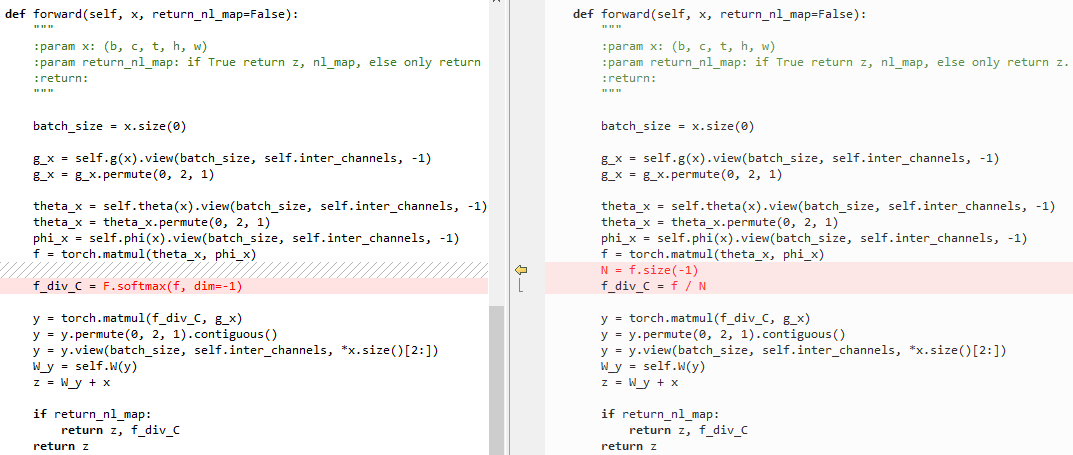
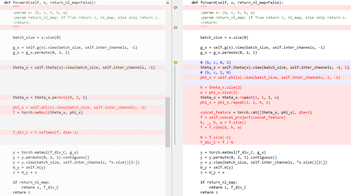
6.2 embedded Gaussian和点乘的区别
点乘代码:
 class _NonLocalBlockND(nn.Module):

     def __init__(self, in_channels, inter_channels=None, dimension=3, sub_sample=True, bn_layer=True):

         super(_NonLocalBlockND, self).__init__()

         assert dimension in [1, 2, 3]

         self.dimension = dimension

         self.sub_sample = sub_sample

         self.in_channels = in_channels

         self.inter_channels = inter_channels

         if self.inter_channels is None:

             self.inter_channels = in_channels // 2

             if self.inter_channels == 0:

                 self.inter_channels = 1

         if dimension == 3:

             conv_nd = nn.Conv3d

             max_pool_layer = nn.MaxPool3d(kernel_size=(1, 2, 2))

             bn = nn.BatchNorm3d

         elif dimension == 2:

             conv_nd = nn.Conv2d

             max_pool_layer = nn.MaxPool2d(kernel_size=(2, 2))

             bn = nn.BatchNorm2d

         else:

             conv_nd = nn.Conv1d

             max_pool_layer = nn.MaxPool1d(kernel_size=(2))

             bn = nn.BatchNorm1d

         self.g = conv_nd(in_channels=self.in_channels, out_channels=self.inter_channels,

                          kernel_size=1, stride=1, padding=0)

         if bn_layer:

             self.W = nn.Sequential(

                 conv_nd(in_channels=self.inter_channels, out_channels=self.in_channels,

                         kernel_size=1, stride=1, padding=0),

                 bn(self.in_channels)

             )

             nn.init.constant_(self.W[1].weight, 0)

             nn.init.constant_(self.W[1].bias, 0)

         else:

             self.W = conv_nd(in_channels=self.inter_channels, out_channels=self.in_channels,

                              kernel_size=1, stride=1, padding=0)

             nn.init.constant_(self.W.weight, 0)

             nn.init.constant_(self.W.bias, 0)

         self.theta = conv_nd(in_channels=self.in_channels, out_channels=self.inter_channels,

                              kernel_size=1, stride=1, padding=0)

         self.phi = conv_nd(in_channels=self.in_channels, out_channels=self.inter_channels,

                            kernel_size=1, stride=1, padding=0)

         if sub_sample:

             self.g = nn.Sequential(self.g, max_pool_layer)

             self.phi = nn.Sequential(self.phi, max_pool_layer)

     def forward(self, x, return_nl_map=False):

         """

         :param x: (b, c, t, h, w)

         :param return_nl_map: if True return z, nl_map, else only return z.

         :return:

         """

         # 令x维度B*C*(K):一维时,x为B*C*(K1);二维时,x为B*C*(K1*K2);三维时,x为B*C*(K1*K2*K3)

         batch_size = x.size(0)

         g_x = self.g(x).view(batch_size, self.inter_channels, -1)    # 通过g函数,并reshape,得到B*inter_channels*(K)矩阵

         g_x = g_x.permute(0, 2, 1)   # 得到B*(K)*inter_channels矩阵,和图2中一致

         theta_x = self.theta(x).view(batch_size, self.inter_channels, -1)   # 通过θ函数,并reshape,得到B*inter_channels*(K)矩阵

         theta_x = theta_x.permute(0, 2, 1)    # 得到B*(K)*inter_channels矩阵,和图2中一致

         phi_x = self.phi(x).view(batch_size, self.inter_channels, -1)    # 通过φ函数,并reshape,得到B*inter_channels*(K)矩阵

         f = torch.matmul(theta_x, phi_x)     # 得到B*(K)*(K)矩阵,和图2中一致

         N = f.size(-1)   # 最后一维的维度

         f_div_C = f / N  # 对最后一维归一化

         y = torch.matmul(f_div_C, g_x)    # 得到B*(K)*inter_channels矩阵,和图2中一致

         y = y.permute(0, 2, 1).contiguous()   # 得到B*inter_channels*(K)矩阵,和图2中一致

         y = y.view(batch_size, self.inter_channels, *x.size()[2:])   # 得到B*inter_channels*(K1或K1*K2或K1*K2*K3)矩阵,和图2中一致

         W_y = self.W(y) # 得到B*C*(K)矩阵,和图2中一致

         z = W_y + x   # 特征图和non local的图相加,得到新的特征图,B*C*(K)

         if return_nl_map:

             return z, f_div_C  # 返回结果及归一化的特征

         return z

 class NONLocalBlock1D(_NonLocalBlockND):

     def __init__(self, in_channels, inter_channels=None, sub_sample=True, bn_layer=True):

         super(NONLocalBlock1D, self).__init__(in_channels,

                                               inter_channels=inter_channels,

                                               dimension=1, sub_sample=sub_sample,

                                               bn_layer=bn_layer)

 class NONLocalBlock2D(_NonLocalBlockND):

     def __init__(self, in_channels, inter_channels=None, sub_sample=True, bn_layer=True):

         super(NONLocalBlock2D, self).__init__(in_channels,

                                               inter_channels=inter_channels,

                                               dimension=2, sub_sample=sub_sample,

                                               bn_layer=bn_layer)

 class NONLocalBlock3D(_NonLocalBlockND):

     def __init__(self, in_channels, inter_channels=None, sub_sample=True, bn_layer=True):

         super(NONLocalBlock3D, self).__init__(in_channels,

                                               inter_channels=inter_channels,

                                               dimension=3, sub_sample=sub_sample,

                                               bn_layer=bn_layer)

 if __name__ == '__main__':

     import torch

     for (sub_sample_, bn_layer_) in [(True, True), (False, False), (True, False), (False, True)]:

         img = torch.zeros(2, 3, 20)

         net = NONLocalBlock1D(3, sub_sample=sub_sample_, bn_layer=bn_layer_)

         out = net(img)

         print(out.size())

         img = torch.zeros(2, 3, 20, 20)

         net = NONLocalBlock2D(3, sub_sample=sub_sample_, bn_layer=bn_layer_)

         out = net(img)

         print(out.size())

         img = torch.randn(2, 3, 8, 20, 20)

         net = NONLocalBlock3D(3, sub_sample=sub_sample_, bn_layer=bn_layer_)

         out = net(img)

         print(out.size())
左侧为embedded Gaussian,右侧为点乘
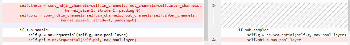
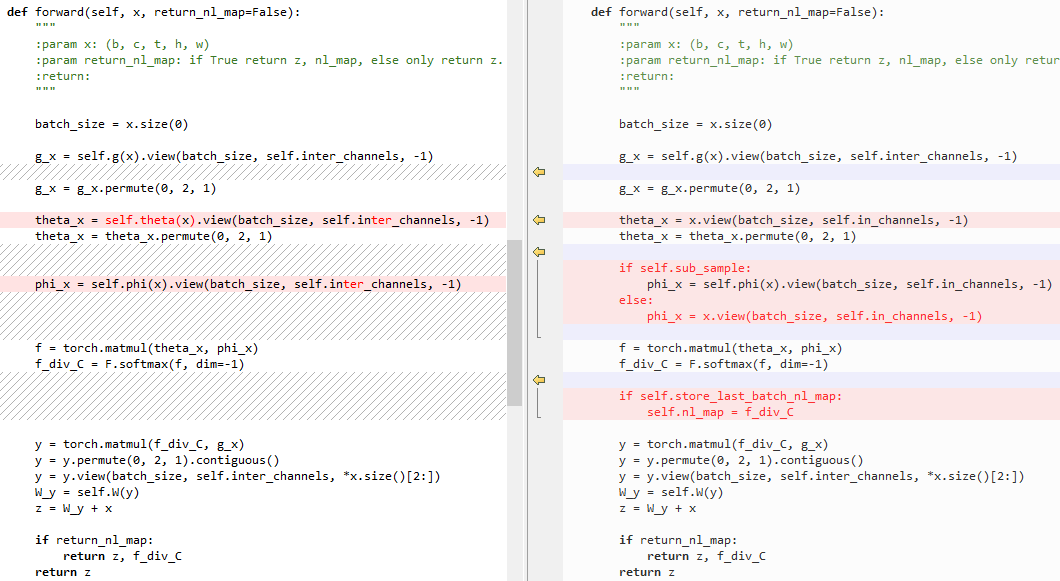
6.3 embedded Gaussian和Gaussian的区别
左侧为embedded Gaussian,右侧为Gaussian
初始化:
forward:
6.4 embedded Gaussian和Concatenation的区别
Concatenation代码:
 class _NonLocalBlockND(nn.Module):

     def __init__(self, in_channels, inter_channels=None, dimension=3, sub_sample=True, bn_layer=True):

         super(_NonLocalBlockND, self).__init__()

         assert dimension in [1, 2, 3]

         self.dimension = dimension

         self.sub_sample = sub_sample

         self.in_channels = in_channels

         self.inter_channels = inter_channels

         if self.inter_channels is None:

             self.inter_channels = in_channels // 2

             if self.inter_channels == 0:

                 self.inter_channels = 1

         if dimension == 3:

             conv_nd = nn.Conv3d

             max_pool_layer = nn.MaxPool3d(kernel_size=(1, 2, 2))

             bn = nn.BatchNorm3d

         elif dimension == 2:

             conv_nd = nn.Conv2d

             max_pool_layer = nn.MaxPool2d(kernel_size=(2, 2))

             bn = nn.BatchNorm2d

         else:

             conv_nd = nn.Conv1d

             max_pool_layer = nn.MaxPool1d(kernel_size=(2))

             bn = nn.BatchNorm1d

         self.g = conv_nd(in_channels=self.in_channels, out_channels=self.inter_channels,

                          kernel_size=1, stride=1, padding=0)

         if bn_layer:

             self.W = nn.Sequential(

                 conv_nd(in_channels=self.inter_channels, out_channels=self.in_channels,

                         kernel_size=1, stride=1, padding=0),

                 bn(self.in_channels)

             )

             nn.init.constant_(self.W[1].weight, 0)

             nn.init.constant_(self.W[1].bias, 0)

         else:

             self.W = conv_nd(in_channels=self.inter_channels, out_channels=self.in_channels,

                              kernel_size=1, stride=1, padding=0)

             nn.init.constant_(self.W.weight, 0)

             nn.init.constant_(self.W.bias, 0)

         self.theta = conv_nd(in_channels=self.in_channels, out_channels=self.inter_channels,

                              kernel_size=1, stride=1, padding=0)

         self.phi = conv_nd(in_channels=self.in_channels, out_channels=self.inter_channels,

                            kernel_size=1, stride=1, padding=0)

         self.concat_project = nn.Sequential(   # 将concat后的特征降维到1维的矩阵

             nn.Conv2d(self.inter_channels * 2, 1, 1, 1, 0, bias=False),

             nn.ReLU()

         )

         if sub_sample:

             self.g = nn.Sequential(self.g, max_pool_layer)

             self.phi = nn.Sequential(self.phi, max_pool_layer)

     def forward(self, x, return_nl_map=False):

         '''

         :param x: (b, c, t, h, w)

         :param return_nl_map: if True return z, nl_map, else only return z.

         :return:

         '''

         # 令x维度B*C*(K):一维时,x为B*C*(K1);二维时,x为B*C*(K1*K2);三维时,x为B*C*(K1*K2*K3)

         batch_size = x.size(0)

         g_x = self.g(x).view(batch_size, self.inter_channels, -1)   # 通过g函数,并reshape,得到B*inter_channels*(K)矩阵

         g_x = g_x.permute(0, 2, 1)  # 得到B*(K)*inter_channels矩阵,和图2中一致

         # (b, c, N, 1)

         theta_x = self.theta(x).view(batch_size, self.inter_channels, -1, 1)  # 通过θ函数,并reshape,得到B*inter_channels*(K)*1矩阵

         # (b, c, 1, N)

         phi_x = self.phi(x).view(batch_size, self.inter_channels, 1, -1) # 通过φ函数,并reshape,得到B*inter_channels*1*(K)矩阵

         h = theta_x.size(2)  # (K)

         w = phi_x.size(3)  # (K)

         theta_x = theta_x.repeat(1, 1, 1, w)  # B*inter_channels*(K)*(K)

         phi_x = phi_x.repeat(1, 1, h, 1)     # B*inter_channels*(K)*(K)

         concat_feature = torch.cat([theta_x, phi_x], dim=1)  # B*(2*inter_channels)*(K)*(K)

         f = self.concat_project(concat_feature)    # B*1*(K)*(K)

         b, _, h, w = f.size()  # B,_,(K),(K)

         f = f.view(b, h, w)   # B*(K)*(K)

         N = f.size(-1)  # (K)

         f_div_C = f / N   # 最后一维归一化,B*(K)*(K)

         y = torch.matmul(f_div_C, g_x)    # 得到B*(K)*inter_channels矩阵,和图2中一致

         y = y.permute(0, 2, 1).contiguous()# 得到B*inter_channels*(K)矩阵,和图2中一致

         y = y.view(batch_size, self.inter_channels, *x.size()[2:])  # 得到B*inter_channels*(K1或K1*K2或K1*K2*K3)矩阵,和图2中一致

         W_y = self.W(y)  # 得到B*C*(K)矩阵,和图2中一致

         z = W_y + x   # 特征图和non local的图相加,得到新的特征图,B*C*(K)

         if return_nl_map:

             return z, f_div_C    # 返回结果及归一化的特征

         return z

 class NONLocalBlock1D(_NonLocalBlockND):

     def __init__(self, in_channels, inter_channels=None, sub_sample=True, bn_layer=True):

         super(NONLocalBlock1D, self).__init__(in_channels,

                                               inter_channels=inter_channels,

                                               dimension=1, sub_sample=sub_sample,

                                               bn_layer=bn_layer)

 class NONLocalBlock2D(_NonLocalBlockND):

     def __init__(self, in_channels, inter_channels=None, sub_sample=True, bn_layer=True):

         super(NONLocalBlock2D, self).__init__(in_channels,

                                               inter_channels=inter_channels,

                                               dimension=2, sub_sample=sub_sample,

                                               bn_layer=bn_layer)

 class NONLocalBlock3D(_NonLocalBlockND):

     def __init__(self, in_channels, inter_channels=None, sub_sample=True, bn_layer=True,):

         super(NONLocalBlock3D, self).__init__(in_channels,

                                               inter_channels=inter_channels,

                                               dimension=3, sub_sample=sub_sample,

                                               bn_layer=bn_layer)

 if __name__ == '__main__':

     import torch

     for (sub_sample_, bn_layer_) in [(True, True), (False, False), (True, False), (False, True)]:

         img = torch.zeros(2, 3, 20)

         net = NONLocalBlock1D(3, sub_sample=sub_sample_, bn_layer=bn_layer_)

         out = net(img)

         print(out.size())

         img = torch.zeros(2, 3, 20, 20)

         net = NONLocalBlock2D(3, sub_sample=sub_sample_, bn_layer=bn_layer_)

         out = net(img)

         print(out.size())

         img = torch.randn(2, 3, 8, 20, 20)

         net = NONLocalBlock3D(3, sub_sample=sub_sample_, bn_layer=bn_layer_)

         out = net(img)

         print(out.size())
左侧为embedded Gaussian,右侧为Concatenation
初始化:

forward:
(原)Non-local Neural Networks的更多相关文章
- Local Binary Convolutional Neural Networks ---卷积深度网络移植到嵌入式设备上?
前言:今天他给大家带来一篇发表在CVPR 2017上的文章. 原文:LBCNN 原文代码:https://github.com/juefeix/lbcnn.torch 本文主要内容:把局部二值与卷积神 ...
- Spurious Local Minima are Common in Two-Layer ReLU Neural Networks
目录 引 主要内容 定理1 推论1 引理1 引理2 Safran I, Shamir O. Spurious Local Minima are Common in Two-Layer ReLU Neu ...
- 论文解读(LA-GNN)《Local Augmentation for Graph Neural Networks》
论文信息 论文标题:Local Augmentation for Graph Neural Networks论文作者:Songtao Liu, Hanze Dong, Lanqing Li, Ting ...
- Deep Learning 16:用自编码器对数据进行降维_读论文“Reducing the Dimensionality of Data with Neural Networks”的笔记
前言 论文“Reducing the Dimensionality of Data with Neural Networks”是深度学习鼻祖hinton于2006年发表于<SCIENCE > ...
- Stanford机器学习---第五讲. 神经网络的学习 Neural Networks learning
原文 http://blog.csdn.net/abcjennifer/article/details/7758797 本栏目(Machine learning)包括单参数的线性回归.多参数的线性回归 ...
- Non-local Neural Networks
1. 摘要 卷积和循环神经网络中的操作都是一次处理一个局部邻域,在这篇文章中,作者提出了一个非局部的操作来作为捕获远程依赖的通用模块. 受计算机视觉中经典的非局部均值方法启发,我们的非局部操作计算某一 ...
- 论文解读二代GCN《Convolutional Neural Networks on Graphs with Fast Localized Spectral Filtering》
Paper Information Title:Convolutional Neural Networks on Graphs with Fast Localized Spectral Filteri ...
- 【转】Artificial Neurons and Single-Layer Neural Networks
原文:written by Sebastian Raschka on March 14, 2015 中文版译文:伯乐在线 - atmanic 翻译,toolate 校稿 This article of ...
- [转]Neural Networks, Manifolds, and Topology
colah's blog Blog About Contact Neural Networks, Manifolds, and Topology Posted on April 6, 2014 top ...
随机推荐
- Docker系列之实战:3.安装MariaDB
环境 [root@centos181001 ~]# cat /etc/centos-release CentOS Linux release 7.6.1810 (Core) [root@centos1 ...
- 多线程的lock功能
import threading def job1(): global A, lock lock.acquire() for i in range(10): A += 1 print('job1', ...
- 剑指offer-18-2. 删除链表中重复的结点
剑指offer-18-2. 删除链表中重复的结点 链表 在一个排序的链表中,存在重复的结点,请删除该链表中重复的结点,重复的结点不保留,返回链表头指针. 例如,链表1->2->3-> ...
- cpupower frequency 无法设置userspace的问题
Disable intel_pstate in grub configure file: $ sudo vi /etc/default/grub Append "intel_pstate=d ...
- app后端用户登录api
app将用户名和密码发送到服务器,服务器验证用户名和密码都正确后,会在redis或memcached服务器中以用户id为键生成token字 符串,然后服务器把token字符串和用户id都返回给客户端( ...
- iPhone7产业链不为人知的辛酸
苹果金秋新品发布会是科技界的"春晚",年复一年地重复,难免会让人产生审美疲劳,但每逢中国教师节前后,全球的科技人士和媒体还是会不约而同地走到一起,等待苹果团队为之奉献出好的产品和 ...
- idea激活教程(永久)支持2019 3.1 亲测
此教程已支持最新2019.3版本 本教程适用Windows.Mac.Ubuntu等所有平台. 激活前准备工作 配置文件修改已经不在bin目录下直接修改,而是通过Idea修改 如果输入code一直弹出来 ...
- CSS——NO.3(CSS选择器)
*/ * Copyright (c) 2016,烟台大学计算机与控制工程学院 * All rights reserved. * 文件名:text.cpp * 作者:常轩 * 微信公众号:Worldhe ...
- C++扬帆远航——12(抓小偷)
/* * Copyright (c) 2016,烟台大学计算机与控制工程学院 * All rights reserved. * 文件名:zhaoxiaotou.cpp * 作者:常轩 * 微信公众号: ...
- 彻底消灭if-else嵌套
一.背景 1.1 反面教材 不知大家有没遇到过像横放着的金字塔一样的if-else嵌套: if (true) { if (true) { if (true) { if (true) { if (tru ...