论文解读（SAGPool）《Self-Attention Graph Pooling》

论文信息

论文标题：Self-Attention Graph Pooling
论文作者：Junhyun Lee, Inyeop Lee, Jaewoo Kang
论文来源：2019, ICML
论文地址：download 
论文代码：download

1 Introduction

　　图池化三种类型：

• • Topology based pooling；
  • Hierarchical pooling；（使用所有从 GNN 获得的节点表示）
  • Hierarchical pooling；

　　关于 Hierarchical pooling 聚类分配矩阵：

　　　　$\begin{array}{j}S^{(l)}=\operatorname{softmax}\left(\mathrm{GNN}_{l}\left(A^{(l)}, X^{(l)}\right)\right) \\A^{(l+1)}=S^{(l) \top} A^{(l)} S^{(l)}\end{array}  \quad\quad\quad\quad(1)$

　　gPool 取得了与 DiffPool 相当的性能，gPool 需要的存储复杂度为 $\mathcal{O}(|V|+|E|)$，而 DiffPool 需要 $\mathcal{O}\left(k|V|^{2}\right)$，其中 $V$、$E$ 和 $k$ 分别表示顶点、边和池化率。gPool 使用一个可学习的向量 $p$ 来计算投影分数，然后使用这些分数来选择排名靠前的节点。投影得分由 $p$ 与所有节点的特征之间的点积得到。这些分数表示可以保留的节点的信息量。下面的公式大致描述了 gPool 中的池化过程：

　　　　$\begin{array}{l} y=X^{(l)} \mathbf{p}^{(l)} /\left\|\mathbf{p}^{(l)}\right\|\\ \mathrm{idx}=\operatorname{top}-\operatorname{rank}(y,\lceil k N\rceil)\\A^{(l+1)}=A_{\mathrm{idx}, \mathrm{idx}}^{(l)}\end{array} \quad\quad\quad\quad(2)$

2 Method

　　框架如下：

　　 

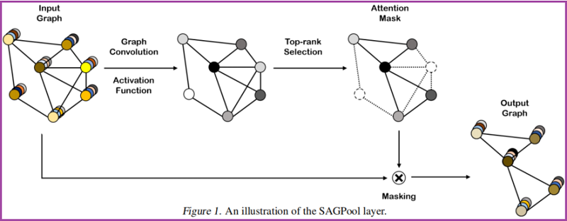
2.1. Self-Attention Graph Pooling

Self-attention mask

　　本文使用图卷积来获得自注意分数：

　　　　$Z=\sigma\left(\tilde{D}^{-\frac{1}{2}} \tilde{A} \tilde{D}^{-\frac{1}{2}} X \Theta_{a t t}\right)  \quad\quad\quad\quad(3)$

　　其中，自注意得分 $Z \in \mathbb{R}^{N \times 1}$、邻接矩阵 $\tilde{A} \in \mathbb{R}^{N \times N}$、注意力参数矩阵 $\Theta_{a t t} \in \mathbb{R}^{F \times 1}$、特征矩阵 $X \in \mathbb{R}^{N \times F}$、度矩阵 $\tilde{D} \in \mathbb{R}^{N \times N}$。

　　这里考虑节点选择方法，即使输入不同大小和结构的图，也会保留输入图的部分节点。

　　　　$\begin{array}{l} \mathrm{idx}=\operatorname{top}-\operatorname{rank}(Z,\lceil k N\rceil)\\Z_{\text {mask }}=Z_{\mathrm{idx}}\end{array}   \quad\quad\quad\quad(4)$

　　基于自注意得分 $Z$ ，选择保留前 $ \lceil k N\rceil$ 个节点，其中 $k \in(0,1]$ 代表着池化率（pooling ratio），$Z_{\text{mask}}$ 是 feature attention mask。。

Graph pooling

　　接着获得新特征矩阵和邻接矩阵：

　　　　 $\begin{array}{l} X^{\prime}=X_{\mathrm{idx},:}\\X_{\text {out }}=X^{\prime} \odot Z_{\text {mask }}\\A_{\text {out }}=A_{\mathrm{idx}, \mathrm{idx}}\end{array} \quad\quad\quad\quad(5)$

　　其中，$\odot$  is the broadcasted elementwise product。

Variation of SAGPool

　　利用图特征矩阵 $X$ 和拓扑结构 $A$ ，计算注意力得分矩阵 $Z$ 的通用形式：

　　　　$Z=\sigma(\operatorname{GNN}(X, A))  \quad\quad\quad\quad(6)$

　　比如 $\text { SAGPool }_{\text {augmentation }}$，加入二跳邻居信息：

　　　　$Z=\sigma\left(\operatorname{GNN}\left(X, A+A^{2}\right)\right)   \quad\quad\quad\quad(7)$

　　比如 $\text { SAGPool }_{\text {serial }}$，堆叠多层 GNN：

　　　　$Z=\sigma\left(\mathrm{GNN}_{2}\left(\sigma\left(\mathrm{GNN}_{1}(X, A)\right), A\right)\right)  \quad\quad\quad\quad(8)$

　　比如 $\text { SAGPool }_{\text {parallel }}$，平均多重注意力分数。$M$ 个 GNN 的平均注意得分如下：

　　　　$Z=\frac{1}{M} \sum_{m} \sigma\left(\mathrm{GNN}_{m}(X, A)\right) \quad\quad\quad\quad(9)$

2.2 Model Architecture

　　本节用来验证模块的有效性。

Convolution layer

　　图卷积 GCN：

　　　　$h^{(l+1)}=\sigma\left(\tilde{D}^{-\frac{1}{2}} \tilde{A} \tilde{D}^{-\frac{1}{2}} h^{(l)} \Theta\right)  \quad\quad\quad\quad(10)$

　　与 $\text{Eq.3}$ 不同的是，$\Theta \in \mathbb{R}^{F \times F^{\prime}}$ 。

Readout layer

　　根据 JK-net architecture 的思想：

　　　　$s=\frac{1}{N} \sum_{i=1}^{N} x_{i} \| \max _{i=1}^{N} x_{i}   \quad\quad\quad\quad(11)$

　　其中：

• • $N$ 代表着节点的个数；
  • $x_{i}$ 代表着第 $i$ 个节点的特征向量；

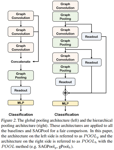
Global pooling architecture & Hierarchical pooling architecture

　　对比如下：

　　

3 Experiments

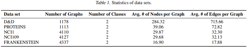
数据集

　　

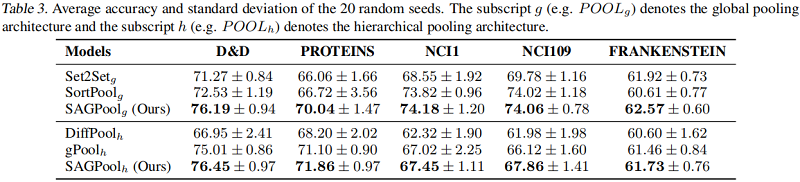
基线实验

　　

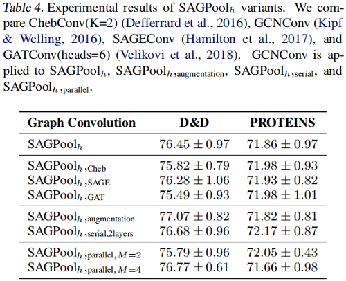
SAGPool 的变体

　　

4 Conclusion

　　本文提出了一种基于自注意的SAGPool图池化方法。我们的方法具有以下特征：分层池、同时考虑节点特征和图拓扑、合理的复杂度和端到端表示学习。SAGPool使用一致数量的参数，而不管输入图的大小如何。我们工作的扩展可能包括使用可学习的池化比率来获得每个图的最优聚类大小，并研究每个池化层中多个注意掩模的影响，其中最终的表示可以通过聚合不同的层次表示来获得。