Pandas系列（十四）- 实战案例

一、series

import pandas as pd
import string
 
#创建Series的两种方式
#方式一
t = pd.Series([1,2,3,4,43],index=list('asdfg'))
print(t)
#方式二
temp_dict = {'name':'xiaohong','age':30,'tel':10086}
t2 = pd.Series(temp_dict)
print(t2)
#字典推导式
a = {string.ascii_uppercase[i]:i for i in range(10)}
print(a)
print(pd.Series(a))
print(pd.Series(a,index=list(string.ascii_uppercase[5:15])))　

二、read_file

import pandas as pd
from pymongo import MongoClient
 
#pandas读取csv文件
# df = pd.read_csv('dogNames2.csv')
# print(df)
 
client = MongoClient()
collection = client['meipai']['meipai_video']
data = collection.find()
data_list = []
for i in data:
    temp = {}
    temp['cut_url'] = i['cut_url']
    temp['create_time'] = i['create_time']
    temp['title'] = i['title']
    temp['video_url'] = i['video_url']
    data_list.append(temp)
 
# print(data)
# t1 = data[0]
# t1 = pd.Series(t1)
# print(t1)
 
df = pd.DataFrame(data_list)
print(df.info())
print(df.describe())
# print(df.head())
# print('*'*100)
# print(df.tail())

　三、dataframe

　　示例一

import pandas as pd
 
temp_dict = {'name':['xiaohong','xiaozhang'],'age':[30,23],'tel':[10086,10010]}
t1 = pd.DataFrame(temp_dict)
print(t1)
 
temp_dict1 = [{'name':'xiaohong','age':23,'tel':10086},{'name':'xiaogang','age':12},{'name':'xiaozhang','tel':10010}]
t2 = pd.DataFrame(temp_dict1)
print(t2)

　　　示例二

import pandas as pd
 
#pandas读取csv文件
df = pd.read_csv('dogNames2.csv')
# print(df.head())
# print(df.info())
 
#DataFrame中排序的方法
df = df.sort_values(by='Count_AnimalName',ascending=False)
# print(df.head())
 
#pandas取行和列的注意事项
# - 方括号写数组，表示取行，对行进行操作
# - 写字符串，表示取列索引，对列进行操作
print(df[:20])
print(df[:20]['Row_Labels'])
print(type(df['Row_Labels']))
 
#bool索引
print(df[(df['Row_Labels'].str.len()>4)&(df['Count_AnimalName']>800)])

　四、电影数据案例

import pandas as pd
from matplotlib import pyplot as plt
 
file_path = './IMDB-Movie-data.csv'
df = pd.read_csv(file_path)
# print(df.head(1))
# print(df.info())
 
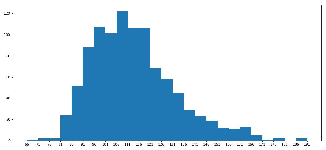
# rating,runtime分布情况
# 选择图形：直方图
# 准备数据
runtime_data = df['Runtime (Minutes)'].values
max_runtime = runtime_data.max()
min_runtime = runtime_data.min()
 
#计算组距
num_bin = (max_runtime-min_runtime)//5
 
#设置图行大小
plt.figure(figsize=(13,6),dpi=80)
#画直方图
plt.hist(runtime_data,num_bin)
 
plt.xticks(range(min_runtime,max_runtime+5,5))
 
#显示
plt.show()

电影案例二

import pandas as pd
from matplotlib import pyplot as plt
from functools import reduce
 
file_path = './IMDB-Movie-data.csv'
df = pd.read_csv(file_path)
# print(df.head(1))
# print(df.info())
 
# rating,runtime分布情况
# 选择图形：直方图
# 准备数据
# runtime_data = df['Runtime (Minutes)'].values
rate_data = df['Rating'].values
max_rate = rate_data.max()
min_rate = rate_data.min()
 
#设置不等宽组距，hist方法中取到的会是一个左闭右开的区间[1,9,3.5)
num_bin_list = [1.9,3.5]
i = 3.5
while i<=max_rate:
    i += 0.5
    num_bin_list.append(i)
print(num_bin_list)
 
#设置图形大小
plt.figure(figsize=(13,6),dpi=80)
#画直方图
plt.hist(rate_data,num_bin_list)
 
#xticks让之前的组距能够对上
plt.xticks(num_bin_list)
 
#显示
plt.show()

　　

[1.9, 3.5, 4.0, 4.5, 5.0, 5.5, 6.0, 6.5, 7.0, 7.5, 8.0, 8.5, 9.0, 9.5]

　五。常用统计方法

import numpy
import pandas as pd
df = pd.read_csv('IMDB-Movie-Data.csv')
print(df.info())
print(df.describe())
#获取评分的均分
rate_mean = df.Rating.mean()
print(rate_mean)
#获取导演的人数
print(df.Director.value_counts().count())
print(len(set(df.Director.tolist())))
print(len(df.Director.unique()))
#获取演员的人数
temp_actors_list = df.Actors.str.split(',').tolist()
actors_list = [i for j in temp_actors_list for i in j]
# numpy.array(temp_actors_list).flatten()
actors_num = len(set(actors_list))
print(actors_num)
<class 'pandas.core.frame.DataFrame'>
RangeIndex: 1000 entries, 0 to 999
Data columns (total 12 columns):
Rank                  1000 non-null int64
Title                 1000 non-null object
Genre                 1000 non-null object
Description           1000 non-null object
Director              1000 non-null object
Actors                1000 non-null object
Year                  1000 non-null int64
Runtime (Minutes)     1000 non-null int64
Rating                1000 non-null float64
Votes                 1000 non-null int64
Revenue (Millions)    872 non-null float64
Metascore             936 non-null float64
dtypes: float64(3), int64(4), object(5)
memory usage: 93.8+ KB
None
              Rank         Year     ...      Revenue (Millions)   Metascore
count  1000.000000  1000.000000     ...              872.000000  936.000000
mean    500.500000  2012.783000     ...               82.956376   58.985043
std     288.819436     3.205962     ...              103.253540   17.194757
min       1.000000  2006.000000     ...                0.000000   11.000000
25%     250.750000  2010.000000     ...               13.270000   47.000000
50%     500.500000  2014.000000     ...               47.985000   59.500000
75%     750.250000  2016.000000     ...              113.715000   72.000000
max    1000.000000  2016.000000     ...              936.630000  100.000000
[8 rows x 7 columns]

　六、统计分类情况

# -*- coding: utf-8 -*-
 
"""
@Datetime: 2018/11/19
@Author: Zhang Yafei
"""
"""
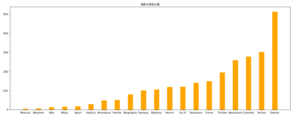
对于这一组电影数据，如果我们希望统计电影分类(genre)的情况，应该如何处理数据？
思路：重新构造一个全为0的数组，列名为分类，如果某一条数据中分类出现过，就让0变为1
"""
import numpy as np
import pandas as pd
from matplotlib import pyplot as plt
from matplotlib import font_manager
 
#中文字体
my_font = font_manager.FontProperties(family='SimHei')
#显示完整的列
pd.set_option('display.max_columns', None)
 
df = pd.read_csv('IMDB-Movie-Data.csv')
#统计分类列表
temp_list = df.Genre.str.split(',').tolist()
genre_list = list(set([i for j in temp_list for i in j]))
 
#构造全为0的数组
zero_df = pd.DataFrame(np.zeros((df.shape[0],len(genre_list))),columns=genre_list)
# print(zero_df)
#给每个电影出现分类的位置赋值1
for i in range(df.shape[0]):
    zero_df.loc[i,temp_list[i]] = 1
 
# print(zero_df.head(1))
genre_count = zero_df.sum(axis=0)
print(genre_count)
 
#排序
genre_count = genre_count.sort_values()
_x = genre_count.index
_y = genre_count.values
#画图
plt.figure(figsize=(15,6),dpi=80)
plt.bar(range(len(_x)),_y,width=0.4,color="orange")
plt.xticks(range(len(_x)),_x)
plt.title('电影分类统计图',fontproperties=my_font)
plt.show()

　　

　七、数据分组与聚合

# -*- coding: utf-8 -*-
 
"""
@Datetime: 2018/11/19
@Author: Zhang Yafei
"""
"""
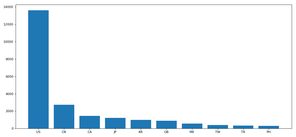
现在我们有一组关于全球星巴克店铺的统计数据，如果我想知道美国的星巴克数量和中国的哪个多，或者我想知道中国每个省份星巴克的数量的情况，那么应该怎么办？
思路：遍历一遍，每次加1 ？？？
"""
import pandas as pd
 
pd.set_option('display.max_columns', None)
 
df = pd.read_csv('starbucks_store_worldwide.csv')
# print(df.head(1))
# print(df.info())
grouped = df.groupby(by='Country')
# print(grouped)
 
# DataFrameGroupBy
# 可以进行遍历
# for i,j in grouped:
#     print(i)
#     print('-'*100)
#     print(j)
#     print('*'*100)
country_count = grouped['Brand'].count()
# print(country_count['US'])
# print(country_count['CN'])
 
#统计中国每个省份店铺的数量
china_data = df[df.Country == 'CN']
china_grouped = china_data.groupby(by='State/Province').count()['Brand']
# print(china_grouped)
#数据按照多个条件进行分组
brand_grouped = df['Brand'].groupby(by=[df['Country'],df['State/Province']]).count()
# print(brand_grouped)
# print(type(brand_grouped))
#数据按照多个条件进行分组,返回dataframe
brand_grouped1 = df[['Brand']].groupby(by=[df['Country'],df['State/Province']]).count()
brand_grouped2 = df.groupby(by=[df['Country'],df['State/Province']])[['Brand']].count()
brand_grouped3 = df.groupby(by=[df['Country'],df['State/Province']]).count()[['Brand']]
# print(brand_grouped1)
# print(brand_grouped2)
# print(brand_grouped3)
#索引的方法和属性
print(brand_grouped1)
print(brand_grouped1.index)

　八、分组聚合

import pandas as pd
from matplotlib import pyplot as plt
 
pd.set_option('display.max_columns', None)
 
df = pd.read_csv('starbucks_store_worldwide.csv')
 
df = df.groupby(by='Country').count()['Brand'].sort_values(ascending=False)[:10]
 
_x = df.index
_y = df.values
 
#画图
plt.figure(figsize=(13,6),dpi=80)
 
plt.bar(_x,_y)
 
plt.show()

　

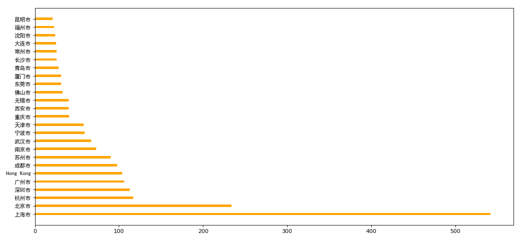
分组聚合二

import pandas as pd
from matplotlib import pyplot as plt
from matplotlib import font_manager
 
my_font = font_manager.FontProperties(family='SimHei')
 
pd.set_option('display.max_columns', None)
 
df = pd.read_csv('starbucks_store_worldwide.csv')
df = df[df['Country']=='CN']
print(df.head(1))
 
df = df.groupby(by='City').count()['Brand'].sort_values(ascending=False)[:25]
 
_x = df.index
_y = df.values
 
#画图
plt.figure(figsize=(13,6),dpi=80)
 
# plt.bar(_x,_y,width=0.3,color='orange')
plt.barh(_x,_y,height=0.3,color='orange')
 
# plt.xticks(_x,fontproperties=my_font)
plt.yticks(_x,fontproperties=my_font)
 
plt.show()

　　

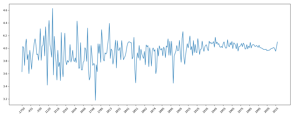
九、book_data

import pandas as pd
from matplotlib import pyplot as plt
 
pd.set_option('display.max_columns', None)
 
df = pd.read_csv('books.csv')
# print(df.info())
data = df[pd.notnull(df['original_publication_year'])]
grouped = data.groupby(by='original_publication_year').count()['title']
# print(grouped)
 
grouped1 = data.average_rating.groupby(by=data['original_publication_year']).mean()
# print(grouped1)
 
_x = grouped1.index
_y = grouped1.values
 
plt.figure(figsize=(15,6),dpi=80)
plt.plot(range(len(_x)),_y)
plt.xticks(range(len(_x))[::10],_x[::10].astype(int),rotation=45)
plt.show()

　　

十、911data

import pandas as pd
from matplotlib import pyplot as plt
import numpy as np
 
pd.set_option('display.max_columns',None)
 
df = pd.read_csv('911.csv')
# print(df.head(1))
# print(df.info())
 
#获取分类
temp_list = df.title.str.split(':').tolist()
cate_list = list(set([i[0] for i in temp_list]))
# print(cate_list)
 
#构造全为0的数组
zeros_df = pd.DataFrame(np.zeros((df.shape[0],len(cate_list))),columns=cate_list)
 
#赋值
for cate in cate_list:
    zeros_df[cate][df.title.str.contains(cate)] = 1
print(zeros_df)
 
sum_ret = zeros_df.sum(axis=0)
print(sum_ret)　　

示例二

import pandas as pd
from matplotlib import pyplot as plt
import numpy as np
 
pd.set_option('display.max_columns',None)
 
df = pd.read_csv('911.csv')
# print(df.head(1))
# print(df.info())
 
#获取分类
temp_list = df.title.str.split(':').tolist()
cate_list = [i[0] for i in temp_list]
 
df['cate'] = pd.DataFrame(np.array(cate_list).reshape(df.shape[0],1))
print(df.groupby(by='cate').count()['title'])　

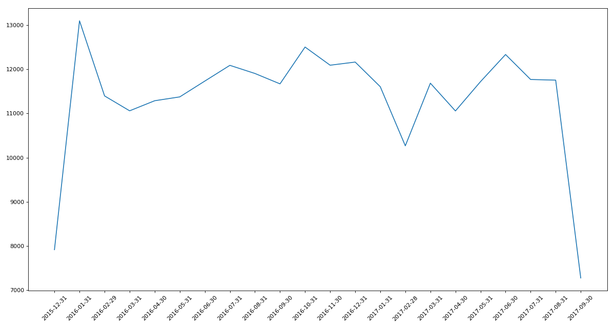
十一、时间序列

实例一

# -*- coding: utf-8 -*-
 
"""
@Datetime: 2018/11/19
@Author: Zhang Yafei
"""
"""
统计出911数据中不同月份电话次数的变化情况
"""
import pandas as pd
from matplotlib import pyplot as plt
import numpy as np
 
pd.set_option('display.max_columns',None)
 
df = pd.read_csv('911.csv')
df.drop_duplicates()
df.timeStamp = pd.to_datetime(df.timeStamp)  #时间字符串转时间格式
 
df.set_index('timeStamp',inplace=True)  #设置时间格式为索引
# print(df.head())
 
#统计出911数据中不同月份电话次数
count_by_month = df.resample('M').count()['title']
print(count_by_month)
 
#画图
_x = count_by_month.index
_y = count_by_month.values
 
plt.figure(figsize=(15,8),dpi=80)
 
plt.plot(range(len(_x)),_y)
 
plt.xticks(range(len(_x)),_x.strftime('%Y-%m-%d'),rotation=45)
 
plt.show()

　　

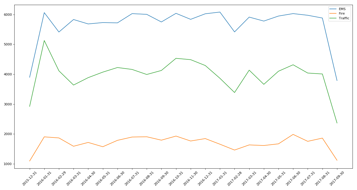
实例二

# -*- coding: utf-8 -*-
 
"""
@Datetime: 2018/11/19
@Author: Zhang Yafei
"""
"""
统计出911数据中不同月份不同类型的电话的次数的变化情况
"""
import pandas as pd
from matplotlib import pyplot as plt
import numpy as np
 
pd.set_option('display.max_columns',None)
 
df = pd.read_csv('911.csv')
#把时间字符串转化为时间类型设置为索引
df.timeStamp = pd.to_datetime(df.timeStamp)
 
#添加列，表示分类
temp_list = df.title.str.split(':').tolist()
cate_list = [i[0] for i in temp_list]
df['cate'] = pd.DataFrame(np.array(cate_list).reshape(df.shape[0],1))
 
df.set_index('timeStamp',inplace=True)
 
plt.figure(figsize=(15, 8), dpi=80)
 
#分组
for group_name,group_data in df.groupby(by='cate'):
    #对不同的分类都进行绘图
    count_by_month = group_data.resample('M').count()['title']
    # 画图
    _x = count_by_month.index
    _y = count_by_month.values
    plt.plot(range(len(_x)),_y,label=group_name)
 
plt.xticks(range(len(_x)), _x.strftime('%Y-%m-%d'), rotation=45)
 
plt.legend(loc='best')
plt.show()

　　

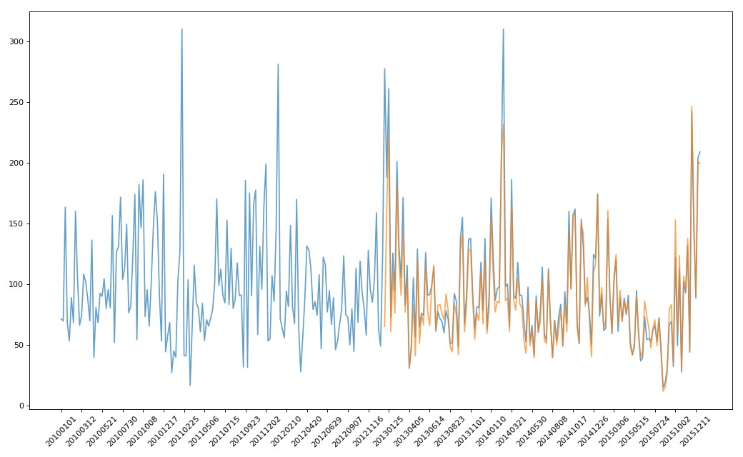
实例三：pm2.5

# -*- coding: utf-8 -*-
 
"""
@Datetime: 2018/11/19
@Author: Zhang Yafei
"""
"""
绘制美国和中国PM2.5随时间的变化情况
"""
import pandas as pd
from matplotlib import pyplot as plt
 
pd.set_option('display.max_columns',None)
 
df = pd.read_csv('PM2.5/BeijingPM20100101_20151231.csv')
# print(df.head())
 
#把分开的时间字符串通过periodIndex的方法转化为pandas的时间类型
period = pd.PeriodIndex(year=df.year,month=df.month,day=df.day,hour=df.hour,freq='H')
df['datetime'] = period
print(df.head(10))
 
#把datetime设置为索引
df.set_index('datetime',inplace=True)
 
#进行降采样
df = df.resample('7D').mean()
 
#处理缺失值，删除缺失数据
# data = df['PM_US Post'].dropna()
# china_data = df['PM_Nongzhanguan'].dropna()
data = df['PM_US Post']
china_data = df['PM_Nongzhanguan']
 
#画图
_x = data.index
_y = data.values
 
_x_china = china_data.index
_y_china = china_data.values
 
plt.figure(figsize=(13,8),dpi=80)
 
plt.plot(range(len(_x)),_y,label='US_POST',alpha=0.7)
plt.plot(range(len(_x_china)),_y_china,label='CN_POST',alpha=0.7)
 
plt.xticks(range(0,len(_x_china),10),list(_x_china.strftime('%Y%m%d'))[::10],rotation=45)
 
plt.show()