机器学习 — 从mnist数据集谈起

　　做了一些简单机器学习任务后，发现必须要对数据集有足够的了解才能动手做一些事，这是无法避免的，否则可能连在干嘛都不知道，而一些官方例程并不会对数据集做过多解释，你甚至连它长什么样都不知道。。。

　　以sklearn的手写数字识别为例，例子中，一句

digits = datasets.load_digits()

　　就拿到数据了，然后又几句

images_and_labels = list(zip(digits.images, digits.target))
for index, (image, label) in enumerate(images_and_labels[:4]):
    plt.subplot(2, 4, index + 1)
    plt.axis('off')
    plt.imshow(image, cmap=plt.cm.gray_r, interpolation='nearest')
    plt.title('Training: %i' % label)

# To apply a classifier on this data, we need to flatten the image, to
# turn the data in a (samples, feature) matrix:
n_samples = len(digits.images)
data = digits.images.reshape((n_samples, -1))

　　就把数据集划分好了，对初学者来说，可能都不知道干了些啥。。。当然更重要的是，跑一边程序看到效果不错，想要用训练好的模型玩玩自己的数据集，却无从下手。。。于是，下面就以这个例子来说一下，如何基本的了解数据集，以及如何构造数据集，或许还会谈谈为什么要这样构造。。。

　　1.认识数据集。

　　看代码，我们发现，该数据集主要由两个部分组成:

　　　　1).images

　　　　2).target

　　target 的划分看起来不复杂，所以可以直接看看其中的部分内容：

>>> print(digits.target.shape)
# (1797,)
>>> print(digits.target[:10])
# [0 1 2 3 4 5 6 7 8 9]
>>> print(digits.target[-10:])
# [5 4 8 8 4 9 0 8 9 8]

　　含义是：target是一个形状为长度为1797的行向量，共有1797个（0~9）数字。

　　images 还需要做一些处理才能使用fit接口，但我们也先看看原本长什么样：

>>> print(digits.image.shape)
# (1797, 8, 8)
>>> print(digits.images[0].shape)
# (8, 8)
>>> print(digits.images[0])
'''
[[ 0.  0.  5. 13.  9.  1.  0.  0.]
 [ 0.  0. 13. 15. 10. 15.  5.  0.]
 [ 0.  3. 15.  2.  0. 11.  8.  0.]
 [ 0.  4. 12.  0.  0.  8.  8.  0.]
 [ 0.  5.  8.  0.  0.  9.  8.  0.]
 [ 0.  4. 11.  0.  1. 12.  7.  0.]
 [ 0.  2. 14.  5. 10. 12.  0.  0.]
 [ 0.  0.  6. 13. 10.  0.  0.  0.]]
'''

　　再画出来看看：

>>> import matplotlib.pyplot as plt
>>> plt.axis('off')
>>> plt.title('label: %i' % digits.target[0])
>>> plt.imshow(digits.images[0], cmap='gray_r')
>>> plt.show()

　　

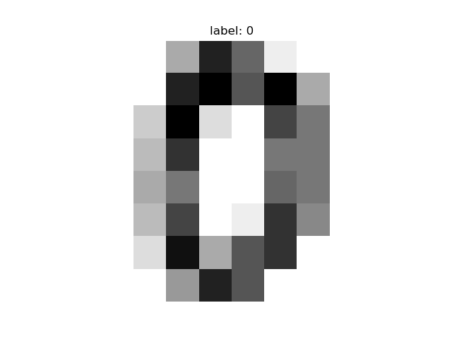
　　含义是：images是由1797张尺寸为8*8的单通道图片组成，而图片内容对应每一张标签的数字的手写数字。

　　于是，这下我们了解了数据集了，但别急，图片集还要做点处理才能使用：

>>> data = digits.images.reshape((n_samples, -1))
>>> print(data.shape)
# (1797, 64)
>>> print(data[0])
'''
[ 0.  0.  5. 13.  9.  1.  0.  0.  0.  0. 13. 15. 10. 15.  5.  0.  0.  3.
 15.  2.  0. 11.  8.  0.  0.  4. 12.  0.  0.  8.  8.  0.  0.  5.  8.  0.
  0.  9.  8.  0.  0.  4. 11.  0.  1. 12.  7.  0.  0.  2. 14.  5. 10. 12.
  0.  0.  0.  0.  6. 13. 10.  0.  0.  0.]
'''

　　把原图片集形状 (numbers, w, h) 变成了 (numbers, w * h)，也就是把2维数组变为一维数组来存储，我个人认为有两个原因，1).算法本身；2).为了性能...处理一维数组的效率比二维数组高很多。（使用深度学习，我们可以利用神经网络自己构造输入形状和输出形状，便利许多。）

　　现在我们很清楚模型要输入什么样的数据才能进行训练了。

　　2.训练模型。

　　该例子使用svm，不同问题的选择不一，而是根据对算法的理解、经验和观察最终训练效果选择合适的算法。

from sklearn import datasets, svm

digits = datasets.load_digits()
n_samples = len(digits.images)
train_x = digits.images.reshape((n_samples, -1))
train_y = digits.target

model = svm.SVC(gamma=0.001)
model.fit(train_x, train_y,)

　　3.评估模型的效果。

from sklearn import metrics

y_real = dateset.target
...
y_pred = model.predict(test_x)
print(metrics.accuracy_score(y_real, y_pred))

　　4.保存和加载模型。

　　保存模型很简单，sklearn有专门提供便利的方法来保存和加载模型：

from sklearn.externals import joblib

joblib.dump(model, 'mnist.m')

　　加载模型：

model = joblib.load('mnist.m')
y_pred = model.predict(test_x)

　　5.最后，部署模型。

　　上面看到，图片的形状必须为8*8像素大小的单通道图片，假如我们有一批50*50的手写数字图片集，想用该模型测试一下效果怎么办，我们只需要改变一下图片分辨率，把形状变为8*8即可。这样，我们才能用自己的数据集来进行测试，或者部署该模型以提供给别人使用。

　　关于如何部署到web，可以参考前一篇随笔。

　　下面是一个例子，使用了一点opencv来把RGB图片转为灰度图、修改图片尺寸以及一些简单的额外处理：

from sklearn import datasets, svm, metrics
import matplotlib.pyplot as plt
from sklearn.externals import joblib
import numpy as np
import cv2 as cv

digits = datasets.load_digits()
n_samples = len(digits.images)
train_x = digits.images.reshape((n_samples, -1))
train_y = digits.target

model = svm.SVC(gamma=0.001)
model.fit(train_x, train_y,)
joblib.dump(model, 'mnist2.m')

w, h = 8, 8
labels = [0, 1, 4, 5]
lenght = len(labels)
images = np.zeros((lenght, h, w), np.uint8)
imgs = []
for i, name in enumerate(labels):
    img = cv.imread('digits/{}.png'.format(name))
    img = cv.resize(img, (h, w), interpolation=cv.INTER_CUBIC)
    for r in range(img.shape[0]):
        for c in range(img.shape[1]):
            img[r, c] = 255 - img[r, c]
    img = cv.cvtColor(img, cv.COLOR_BGR2GRAY)
    imgs.append(img)
    images[i] = img
images = images / 255.0
images = images.reshape((lenght, -1))
pred = model.predict(images)
print(metrics.accuracy_score(labels, pred))
for index, (image, label) in enumerate(list(zip(imgs, pred))):
    plt.subplot(1, lenght, index + 1)
    plt.axis('off')
    plt.imshow(image, cmap='gray_r', interpolation='nearest')
    plt.title('pred: %i' % label)
plt.show()

　　嘛，虽然最后结果很糟。。4张图片识别率只有25%，唯一一张识别成功的，还是因为数据全部被识别为1，具体也不知道为啥，我想是因为我弄的数据集的问题。。。

　　6.使用深度学习

　　再来扩展一下，这次换一种方式来看看是如何处理的（依然使用sklearn提供的数据集）。

　　1).稍微老式一点的方法来处理，基本原理 $ y = Wx + b $，求解这个线性方程组，y是一个独热编码的列向量，W是权重系数矩阵，x是图像，b是偏移量，模型训练过程利用了梯度下降来学习 W 和 b（参考：http://tensorfly.cn/tfdoc/tutorials/mnist_pros.html）

# from keras import *
import tensorflow as tf
import matplotlib.pyplot as plt
import numpy as np
from sklearn import datasets
from sklearn.preprocessing import OneHotEncoder

dataset = datasets.load_digits()
n_samples = len(dataset.images)
images = dataset.images.reshape((n_samples, -1))
train_x = images[:n_samples//2]
test_x = images[n_samples//2:]
digits = np.array([0, 1, 2, 3, 4, 5, 6, 7, 8, 9])
digits = digits.reshape((10, 1))
onehot = OneHotEncoder()
onehot.fit(digits)
label = [onehot.transform([[_]]).toarray()[0] for _ in dataset.target]
train_y = label[:n_samples//2]
test_y = label[n_samples//2:]
x = tf.placeholder('float', [None, 64])
y_ = tf.placeholder('float', [None, 10])
W = tf.Variable(tf.zeros([64, 10]))
b = tf.Variable(tf.zeros([10]))
y = tf.nn.softmax(tf.matmul(x, W) + b)
cross_entropy = -tf.reduce_sum(y_*tf.log(y))
train_step = tf.train.GradientDescentOptimizer(learning_rate=0.15).minimize(cross_entropy)
sess = tf.Session()
sess.run(tf.global_variables_initializer())
sess.run(train_step, feed_dict={x: train_x, y_: train_y})
correct_prediction = tf.equal(tf.argmax(y, 1), tf.argmax(y_, 1))
accuracy = tf.reduce_mean(tf.cast(correct_prediction, "float"))
print(sess.run(accuracy, feed_dict={x: test_x, y_: test_y}))
pred = sess.run(y, feed_dict={x: test_x})
print(pred)

　　准确率：

0.77864295

　　2).tensorflow还有更便利的办法构建网络层，我们可以自己定义输入形状和输出形状，不需要对数据集做太多处理，也不用对标签进行独热编码了（参考：https://www.tensorflow.org/tutorials/)：

# from keras import *
import tensorflow as tf
import matplotlib.pyplot as plt
import numpy as np
from sklearn import datasets
from sklearn.preprocessing import OneHotEncoder

dataset = datasets.load_digits()
n_samples = len(dataset.images)
sizes = n_samples // 2

train_x = dataset.images[:sizes] / 255.0
test_x = dataset.images[sizes:] / 255.0
train_y = dataset.target[:sizes]
test_y = dataset.target[sizes:]

model = tf.keras.Sequential([
    tf.keras.layers.Flatten(input_shape=(8, 8)),
    tf.keras.layers.Dense(512, activation=tf.nn.relu),
    tf.keras.layers.Dropout(0.2),
    tf.keras.layers.Dense(10, activation=tf.nn.softmax)
])

model.compile(optimizer='adam', loss='sparse_categorical_crossentropy', metrics=['accuracy'])
model.fit(train_x, train_y, epochs=10)
test_loss, test_acc = model.evaluate(test_x, test_y)
print(test_acc)

y_pred = model.predict(test_x)
y_pred = [np.argmax(_) for _ in y_pred]

for i, (image, real, pred) in enumerate(zip(test_x[:12], test_y[:12], y_pred[:12])):
    plt.subplot(3, 4, i + 1)
    plt.title('real:{} pred:{}'.format(real, pred))
    plt.axis('off')
    plt.imshow(image, cmap='gray_r')
plt.show()

　　跑了几次，选了一个准确率稍微好看一点的：

0.8331479422242544

　　看看测试集的前12个预测结果如何：

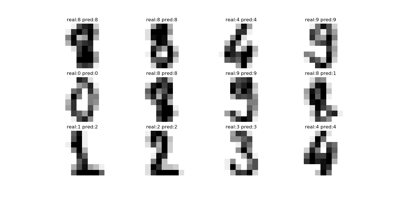
　　当然准确率还可以再优化。

　　然后，我用所有sklearn的digits数据集训练了一个准确率93%的模型来测试我自己弄的数据：

import numpy as np
import matplotlib.pyplot as plt
import cv2 as cv

target = [0, 1, 4, 5]
images = np.zeros((4, 8, 8), np.uint8)
imgs = []
for _, i in enumerate(target):
    img = cv.imread('digits/%i.png' % i)
    img = cv.resize(img, (8, 8), interpolation=cv.INTER_CUBIC)
    for r in range(img.shape[0]):
        for c in range(img.shape[1]):
            img[r, c] = 255 - img[r, c]
    img = cv.cvtColor(img, cv.COLOR_BGR2GRAY)
    # img = cv.Laplacian(img, cv.CV_64F)
    imgs.append(img)
    images[_] = img
model = tf.keras.models.load_model('mnist.h5')
model.compile(optimizer='adam', loss='sparse_categorical_crossentropy', metrics=['accuracy'])
y_pred = model.predict(images)
loss, acc = model.evaluate(images, target)
print(acc)
y_pred = [np.argmax(_) for _ in y_pred]
for i, (image, real, pred) in enumerate(zip(imgs, target, y_pred)):
    plt.subplot(1, 4, i + 1)
    plt.title('real:{} pred:{}'.format(real, pred))
    plt.axis('off')
    plt.imshow(image, cmap='gray_r')
plt.show()

　　只有4张图，准确率50%

　　效果：

　　# 2018-12-02

　　今天又换了一批数据集（训练集60000张，测试集10000张）使用sklearn的svm来训练了一个在测试集上准确率表现为94%的模型，来识别我的那4张。

　　训练代码如下：

import tensorflow as tf
import numpy as np
import matplotlib.pyplot as plt
import cv2 as cv
from sklearn import svm, metrics
from sklearn.externals import joblib

mnist = tf.keras.datasets.mnist
(x_train, y_train), (x_test, y_test) = mnist.load_data()
x_train, x_test = x_train / 255.0, x_test / 255.0

# print(x_train.shape, y_train.shape)

x_train = x_train.reshape((60000, -1))
x_test = x_test.reshape((10000, -1))

model = svm.SVC(gamma=0.001)
model.fit(x_train, y_train)
joblib.dump(model, 'mnist.m')

y_pred = model.predict(x_test)
print(metrics.accuracy_score(y_test, y_pred))

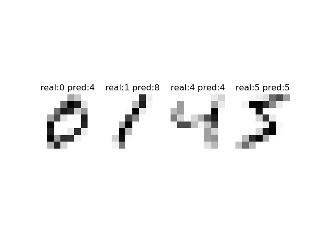
　　然后测试我的数据集：

import tensorflow as tf
import numpy as np
import matplotlib.pyplot as plt
import cv2 as cv
from sklearn import svm, metrics, datasets
from sklearn.externals import joblib

y_test = [0, 1, 4, 5]
x_test = np.zeros((4, 28, 28), np.uint8)
imgs = []
for _, i in enumerate(y_test):
    img = cv.imread('digits/%i.png' % i)
    img = cv.resize(img, (28, 28), interpolation=cv.INTER_CUBIC)
    for r in range(img.shape[0]):
        for c in range(img.shape[1]):
            img[r, c] = 255 - img[r, c]
    img = cv.cvtColor(img, cv.COLOR_BGR2GRAY)
    imgs.append(img)
    x_test[_] = img
x_test = x_test / 255.0
x_test = x_test.reshape((4, -1))

model = joblib.load('mnist.m')
print('loaded model')
y_pred = model.predict(x_test)
print(metrics.accuracy_score(y_test, y_pred))

for index, (image, real, pred) in enumerate(zip(imgs, y_test, y_pred)):
    plt.subplot(1, 4, index + 1)
    plt.axis('off')
    plt.imshow(image, cmap='gray_r', interpolation='nearest')
    plt.title('real:{} pred:{}'.format(real, pred))
plt.show()

　　准确率也是50%，之前没有加

x_test = x_test / 255.0

　　这句时，会全部识别为同一个数字。。。

　　AutoML可以看看：https://qiita.com/Hironsan/items/30fe09c85da8a28ebd63