DSP using MATLAB 示例Example3.9

用到的性质

上代码：

n = 0:100; x = cos(pi*n/2);
k = -100:100; w = (pi/100)*k;                 % freqency between -pi and +pi  ,   [0,pi] axis divided into 101 points.
X = x * (exp(-j*pi/100)) .^ (n'*k);           % DTFT of x

% signal multiplied
y = exp(j*pi*n/4) .* x;                    % signal multiplied by exp(j*pi*n*4)
Y = y * (exp(-j*pi/100)) .^ (n'*k);        % DTFT of y 

magX = abs(X); angX = angle(X); realX = real(X); imagX = imag(X);
magY = abs(Y); angY = angle(Y); realY = real(Y); imagY = imag(Y);

%verification
%Y_check = (exp(-j*2) .^ w) .* X;             % multiplication by exp(-j2w)
%error = max(abs(Y-Y_check));                 % Difference

figure('NumberTitle', 'off', 'Name', 'x & y sequence')
set(gcf,'Color','white');
subplot(2,1,1); stem(n,x); title('x=cos(\pin/2) sequence');             xlabel('n'); ylabel('x(n)'); grid on;
subplot(2,1,2); stem(n,y); title('y=exp(j\pin/4)cos(\pin/2) sequence'); xlabel('n'); ylabel('y(n)'); grid on;

%% --------------------------------------------------------------
%%        START X's  mag ang real imag
%% --------------------------------------------------------------
figure('NumberTitle', 'off', 'Name', 'X its Magnitude and Angle, Real and Imaginary Part');
set(gcf,'Color','white');
subplot(2,2,1); plot(w/pi,magX); grid on;  % axis([-2,2,0,15]);
title('Magnitude Part');
xlabel('frequency in \pi units'); ylabel('Magnitude  |X|');
subplot(2,2,3); plot(w/pi, angX/pi); grid on;  % axis([-2,2,-1,1]);
title('Angle Part');
xlabel('frequency in \pi units'); ylabel('Radians/\pi');

subplot('2,2,2'); plot(w/pi, realX); grid on;
title('Real Part');
xlabel('frequency in \pi units'); ylabel('Real');
subplot('2,2,4'); plot(w/pi, imagX); grid on;
title('Imaginary Part');
xlabel('frequency in \pi units'); ylabel('Imaginary');
%% --------------------------------------------------------------
%%        END X's  mag ang real imag
%% --------------------------------------------------------------

%% --------------------------------------------------------------
%%        START Y's  mag ang real imag
%% --------------------------------------------------------------
figure('NumberTitle', 'off', 'Name', 'Y its Magnitude and Angle, Real and Imaginary Part');
set(gcf,'Color','white');
subplot(2,2,1); plot(w/pi,magY); grid on;  % axis([-2,2,0,15]);
title('Magnitude Part');
xlabel('frequency in \pi units'); ylabel('Magnitude  |Y|');
subplot(2,2,3); plot(w/pi, angY/pi); grid on;  % axis([-2,2,-1,1]);
title('Angle Part');
xlabel('frequency in \pi units'); ylabel('Radians/\pi');

subplot('2,2,2'); plot(w/pi, realY); grid on;
title('Real Part');
xlabel('frequency in \pi units'); ylabel('Real');
subplot('2,2,4'); plot(w/pi, imagY); grid on;
title('Imaginary Part');
xlabel('frequency in \pi units'); ylabel('Imaginary');

%% --------------------------------------------------------------
%%        END Y's  mag ang real imag
%% --------------------------------------------------------------

%% ----------------------------------------------------------------
%%        START Graphical verification
%% ----------------------------------------------------------------
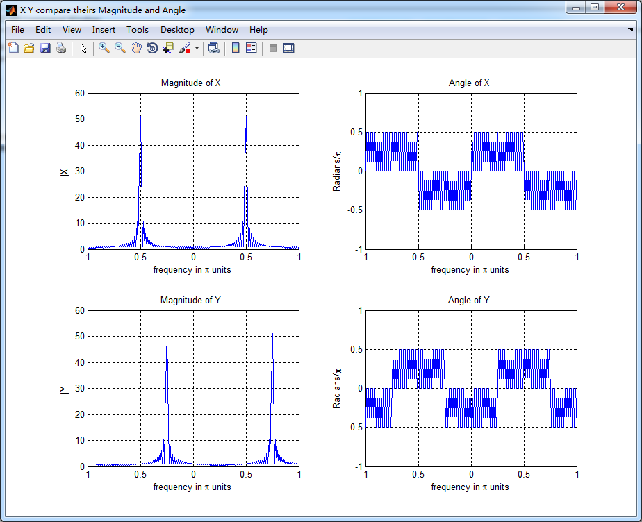
figure('NumberTitle', 'off', 'Name', 'X Y compare theirs Magnitude and Angle');
set(gcf,'Color','white');
subplot(2,2,1); plot(w/pi,magX); grid on; axis([-1,1,0,60]);
xlabel('frequency in \pi units'); ylabel('|X|'); title('Magnitude of X ');
subplot(2,2,2); plot(w/pi,angX/pi); grid on; axis([-1,1,-1,1]);
xlabel('frequency in \pi units'); ylabel('Radians/\pi'); title('Angle of X ');

subplot(2,2,3); plot(w/pi,magY); grid on; axis([-1,1,0,60]);
xlabel('frequency in \pi units'); ylabel('|Y|'); title('Magnitude of Y ');
subplot(2,2,4); plot(w/pi,angY/pi); grid on; axis([-1,1,-1,1]);
xlabel('frequency in \pi units'); ylabel('Radians/\pi'); title('Angle of Y ');

%% ----------------------------------------------------------------
%%        END Graphical verification
%% ----------------------------------------------------------------

运行结果：