scikit-learn机器学习(三)多项式回归(二阶，三阶，九阶)

我们仍然使用披萨直径的价格的数据

import matplotlib

matplotlib.rcParams['font.sans-serif']=[u'simHei']

matplotlib.rcParams['axes.unicode_minus']=False

import numpy as np

import pandas as pd

import matplotlib.pyplot as plt

from sklearn.linear_model import LinearRegression

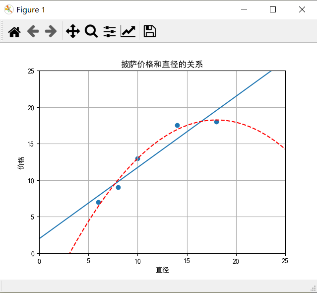
from sklearn.preprocessing import PolynomialFeatures

X_train = [[6],[8],[10],[14],[18]]

y_train = [[7],[9],[13],[17.5],[18]]

X_test = [[6],[8],[11],[16]]

y_test = [[8],[12],[15],[18]]

LR = LinearRegression()

LR.fit(X_train,y_train)

xx = np.linspace(0,26,100)

yy = LR.predict(xx.reshape(xx.shape[0],1))

plt.plot(xx,yy)

二阶多项式回归

# In[1] 二次回归，二阶多项式回归

#PolynomialFeatures转换器可以用于为一个特征表示增加多项式特征

quadratic_featurizer = PolynomialFeatures(degree=2)

X_train_quadratic = quadratic_featurizer.fit_transform(X_train)

X_test_quadratic = quadratic_featurizer.transform(X_test)

regressor_quadratic = LinearRegression()

regressor_quadratic.fit(X_train_quadratic,y_train)

xx_quadratic = quadratic_featurizer.transform(xx.reshape(xx.shape[0],1))

yy_quadratic = regressor_quadratic.predict(xx_quadratic)

plt.plot(xx,yy_quadratic,c='r',linestyle='--')

# In[2] 图参数，输出结果

plt.title("披萨价格和直径的关系")

plt.xlabel("直径")

plt.ylabel("价格")

plt.axis([0,25,0,25])

plt.grid(True)

plt.scatter(X_train,y_train)

print("X_train\n",X_train)

print("X_train_quadratic\n",X_train_quadratic)

print("X_test\n",X_test)

print("X_test_quadratic\n",X_test_quadratic)

print("简单线性规划R方",LR.score(X_test,y_test))

print("二阶多项式回归R方",regressor_quadratic.score(X_test_quadratic,y_test))

X_train

 [[6], [8], [10], [14], [18]]

X_train_quadratic

 [[  1.   6.  36.]

 [  1.   8.  64.]

 [  1.  10. 100.]

 [  1.  14. 196.]

 [  1.  18. 324.]]

X_test

 [[6], [8], [11], [16]]

X_test_quadratic

 [[  1.   6.  36.]

 [  1.   8.  64.]

 [  1.  11. 121.]

 [  1.  16. 256.]]

简单线性规划R方 0.809726797707665

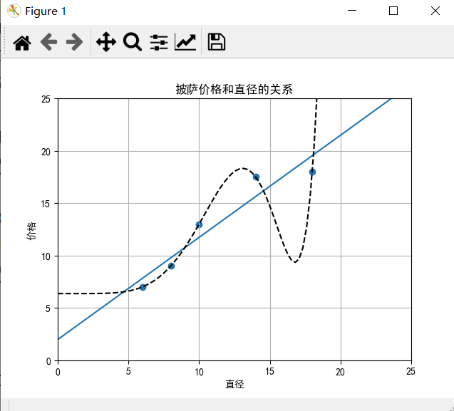
三阶多项式回归

# In[3] 尝试三阶多项式回归

cubic_featurizer = PolynomialFeatures(degree=3)

X_train_cubic = cubic_featurizer.fit_transform(X_train)

X_test_cubic = cubic_featurizer.transform(X_test)

regressor_cubic = LinearRegression()

regressor_cubic.fit(X_train_cubic,y_train)

xx_cubic = cubic_featurizer.transform(xx.reshape(xx.shape[0],1))

yy_cubic = regressor_cubic.predict(xx_cubic)

plt.plot(xx,yy_cubic,c='g',linestyle='--')

plt.show()

print("X_train\n",X_train)

print("X_train_cubic\n",X_train_cubic)

print("X_test\n",X_test)

print("X_test_cubic\n",X_test_cubic)

print("三阶多项式回归R方",regressor_cubic.score(X_test_cubic,y_test))

X_train

 [[6], [8], [10], [14], [18]]

X_train_cubic

 [[1.000e+00 6.000e+00 3.600e+01 2.160e+02]

 [1.000e+00 8.000e+00 6.400e+01 5.120e+02]

 [1.000e+00 1.000e+01 1.000e+02 1.000e+03]

 [1.000e+00 1.400e+01 1.960e+02 2.744e+03]

 [1.000e+00 1.800e+01 3.240e+02 5.832e+03]]

X_test

 [[6], [8], [11], [16]]

X_test_cubic

 [[1.000e+00 6.000e+00 3.600e+01 2.160e+02]

 [1.000e+00 8.000e+00 6.400e+01 5.120e+02]

 [1.000e+00 1.100e+01 1.210e+02 1.331e+03]

 [1.000e+00 1.600e+01 2.560e+02 4.096e+03]]

三阶多项式回归R方 0.8356924156036954

九阶多项式回归

# In[4] 尝试九阶多项式回归

nine_featurizer = PolynomialFeatures(degree=9)

X_train_nine = nine_featurizer.fit_transform(X_train)

X_test_nine = nine_featurizer.transform(X_test)

regressor_nine = LinearRegression()

regressor_nine.fit(X_train_nine,y_train)

xx_nine = nine_featurizer.transform(xx.reshape(xx.shape[0],1))

yy_nine = regressor_nine.predict(xx_nine)

plt.plot(xx,yy_nine,c='k',linestyle='--')

plt.show()

print("X_train\n",X_train)

print("X_train_nine\n",X_train_nine)

print("X_test\n",X_test)

print("X_test_nine\n",X_test_nine)

print("九阶多项式回归R方",regressor_nine.score(X_test_nine,y_test))

X_train

 [[6], [8], [10], [14], [18]]

X_train_nine

 [[1.00000000e+00 6.00000000e+00 3.60000000e+01 2.16000000e+02

  1.29600000e+03 7.77600000e+03 4.66560000e+04 2.79936000e+05

  1.67961600e+06 1.00776960e+07]

 [1.00000000e+00 8.00000000e+00 6.40000000e+01 5.12000000e+02

  4.09600000e+03 3.27680000e+04 2.62144000e+05 2.09715200e+06

  1.67772160e+07 1.34217728e+08]

 [1.00000000e+00 1.00000000e+01 1.00000000e+02 1.00000000e+03

  1.00000000e+04 1.00000000e+05 1.00000000e+06 1.00000000e+07

  1.00000000e+08 1.00000000e+09]

 [1.00000000e+00 1.40000000e+01 1.96000000e+02 2.74400000e+03

  3.84160000e+04 5.37824000e+05 7.52953600e+06 1.05413504e+08

  1.47578906e+09 2.06610468e+10]

 [1.00000000e+00 1.80000000e+01 3.24000000e+02 5.83200000e+03

  1.04976000e+05 1.88956800e+06 3.40122240e+07 6.12220032e+08

  1.10199606e+10 1.98359290e+11]]

X_test

 [[6], [8], [11], [16]]

X_test_nine

 [[1.00000000e+00 6.00000000e+00 3.60000000e+01 2.16000000e+02

  1.29600000e+03 7.77600000e+03 4.66560000e+04 2.79936000e+05

  1.67961600e+06 1.00776960e+07]

 [1.00000000e+00 8.00000000e+00 6.40000000e+01 5.12000000e+02

  4.09600000e+03 3.27680000e+04 2.62144000e+05 2.09715200e+06

  1.67772160e+07 1.34217728e+08]

 [1.00000000e+00 1.10000000e+01 1.21000000e+02 1.33100000e+03

  1.46410000e+04 1.61051000e+05 1.77156100e+06 1.94871710e+07

  2.14358881e+08 2.35794769e+09]

 [1.00000000e+00 1.60000000e+01 2.56000000e+02 4.09600000e+03

  6.55360000e+04 1.04857600e+06 1.67772160e+07 2.68435456e+08

  4.29496730e+09 6.87194767e+10]]

九阶多项式回归R方 -0.09435666704291412

所有代码

# -*- coding: utf-8 -*-

import matplotlib

matplotlib.rcParams['font.sans-serif']=[u'simHei']

matplotlib.rcParams['axes.unicode_minus']=False

import numpy as np

import pandas as pd

import matplotlib.pyplot as plt

from sklearn.linear_model import LinearRegression

from sklearn.preprocessing import PolynomialFeatures

X_train = [[6],[8],[10],[14],[18]]

y_train = [[7],[9],[13],[17.5],[18]]

X_test = [[6],[8],[11],[16]]

y_test = [[8],[12],[15],[18]]

LR = LinearRegression()

LR.fit(X_train,y_train)

xx = np.linspace(0,26,100)

yy = LR.predict(xx.reshape(xx.shape[0],1))

plt.plot(xx,yy)

# In[1] 二次回归，二阶多项式回归

#PolynomialFeatures转换器可以用于为一个特征表示增加多项式特征

quadratic_featurizer = PolynomialFeatures(degree=2)

X_train_quadratic = quadratic_featurizer.fit_transform(X_train)

X_test_quadratic = quadratic_featurizer.transform(X_test)

regressor_quadratic = LinearRegression()

regressor_quadratic.fit(X_train_quadratic,y_train)

xx_quadratic = quadratic_featurizer.transform(xx.reshape(xx.shape[0],1))

yy_quadratic = regressor_quadratic.predict(xx_quadratic)

plt.plot(xx,yy_quadratic,c='r',linestyle='--')

# In[2] 图参数，输出结果

plt.title("披萨价格和直径的关系")

plt.xlabel("直径")

plt.ylabel("价格")

plt.axis([0,25,0,25])

plt.grid(True)

plt.scatter(X_train,y_train)

print("X_train\n",X_train)

print("X_train_quadratic\n",X_train_quadratic)

print("X_test\n",X_test)

print("X_test_quadratic\n",X_test_quadratic)

print("简单线性规划R方",LR.score(X_test,y_test))

print("二阶多项式回归R方",regressor_quadratic.score(X_test_quadratic,y_test))

# In[3] 尝试三阶多项式回归

cubic_featurizer = PolynomialFeatures(degree=3)

X_train_cubic = cubic_featurizer.fit_transform(X_train)

X_test_cubic = cubic_featurizer.transform(X_test)

regressor_cubic = LinearRegression()

regressor_cubic.fit(X_train_cubic,y_train)

xx_cubic = cubic_featurizer.transform(xx.reshape(xx.shape[0],1))

yy_cubic = regressor_cubic.predict(xx_cubic)

plt.plot(xx,yy_cubic,c='g',linestyle='--')

plt.show()

print("X_train\n",X_train)

print("X_train_cubic\n",X_train_cubic)

print("X_test\n",X_test)

print("X_test_cubic\n",X_test_cubic)

print("三阶多项式回归R方",regressor_cubic.score(X_test_cubic,y_test))

# In[4] 尝试九阶多项式回归

nine_featurizer = PolynomialFeatures(degree=9)

X_train_nine = nine_featurizer.fit_transform(X_train)

X_test_nine = nine_featurizer.transform(X_test)

regressor_nine = LinearRegression()

regressor_nine.fit(X_train_nine,y_train)

xx_nine = nine_featurizer.transform(xx.reshape(xx.shape[0],1))

yy_nine = regressor_nine.predict(xx_nine)

plt.plot(xx,yy_nine,c='k',linestyle='--')

plt.show()

print("X_train\n",X_train)

print("X_train_nine\n",X_train_nine)

print("X_test\n",X_test)

print("X_test_nine\n",X_test_nine)

print("九阶多项式回归R方",regressor_nine.score(X_test_nine,y_test))

scikit-learn机器学习(三)多项式回归(二阶，三阶，九阶)的更多相关文章

(原创)（三）机器学习笔记之Scikit Learn的线性回归模型初探
一.Scikit Learn中使用estimator三部曲 1. 构造estimator 2. 训练模型:fit 3. 利用模型进行预测:predict 二.模型评价模型训练好后,度量模型拟合效果的 ...
Scikit Learn: 在python中机器学习
转自:http://my.oschina.net/u/175377/blog/84420#OSC_h2_23 Scikit Learn: 在python中机器学习 Warning 警告:有些没能理解的 ...
(原创)（四）机器学习笔记之Scikit Learn的Logistic回归初探
目录 5.3 使用LogisticRegressionCV进行正则化的 Logistic Regression 参数调优一.Scikit Learn中有关logistics回归函数的介绍 1. 交叉 ...
scikit learn 模块调参 pipeline+girdsearch 数据举例：文档分类（python代码）
scikit learn 模块调参 pipeline+girdsearch 数据举例:文档分类数据集 fetch_20newsgroups #-*- coding: UTF-8 -*- import ...
TensorFlow 便捷的实现机器学习三
TensorFlow 便捷的实现机器学习三 MNIST 卷积神经网络 Fly Overview Enabling Logging with TensorFlow Configuring a Vali ...
【机器学习】多项式回归sklearn实现
[机器学习]多项式回归原理介绍 [机器学习]多项式回归python实现 [机器学习]多项式回归sklearn实现使用sklearn框架实现多项式回归.使用框架更方便,可以少写很多代码. 使用一个简单 ...
【机器学习】多项式回归python实现
[机器学习]多项式回归原理介绍 [机器学习]多项式回归python实现 [机器学习]多项式回归sklearn实现使用python实现多项式回归,没有使用sklearn等机器学习框架,目的是帮助理解算 ...
Scikit Learn
Scikit Learn Scikit-Learn简称sklearn,基于 Python 语言的,简单高效的数据挖掘和数据分析工具,建立在 NumPy,SciPy 和 matplotlib 上.
机器学习框架Scikit Learn的学习
一安装安装pip 代码如下:# wget "https://pypi.python.org/packages/source/p/pip/pip-1.5.4.tar.gz#md5=83 ...

随机推荐

学JAVA有哪些好的技巧方法？干货分享
作为编程语言届的老大哥,学习JAVA的人数不胜数,在这里分享一些学习JAVA的技巧以及方法,当然,这些技巧及方法使用范围包含但不限于JAVA. ① 笔记软件印象笔记:多端互通很方便(https:// ...
linux（3）
一.用户和组的管理 Linux/Unix是多用户系统: root是超级用户,拥有最高权限.其它用户及权限由root来管理.对比Windows系统: 控制面板 -> 管理工具 -> 计算机管 ...
Petrozavodsk Winter Training Camp 2018 Jagiellonian U Contest Problem A. XOR
先把所有的数异或起来得到sum 然后sum有一些位是1一些位是0 是0的位表示所有数里面有这位的数是偶数个则无论怎么划分数这一位对最终的答案都是不会有贡献的因为偶数=偶数+偶数/奇数+奇数 ...
Java多维数组定义以及常见异常
import java.lang.*; import java.util.*; public class Demo1 { public static void main(String args[]){ ...
js获取文件后缀名
function extname(filename){ if(!filename||typeof filename!='string'){ return false }; let a = filena ...
Flask实现简单的群聊和单聊
Flask是使用python写的一个简单轻量级的框架,今天我们使用Flask实现一个简单的单聊和群聊功能 . 主要思路 : 前端登录聊天室,聊天室信息包含用户的登录信息,相当于一个登录功能,会把这个信 ...
洛谷P1339 热浪【最短路】
题目:https://www.luogu.org/problemnew/show/P1339 题意:给定一张图,问起点到终点的最短路. 思路:dijkstra板子题. 很久没有写最短路了.总结一下di ...
BZOJ 4864: [BeiJing 2017 Wc]神秘物质 (块状链表/平衡树 )
这就是一道数据结构裸题啊,最大极差就是区间最大值减最小值,最小极差就是相邻两个数差的最小值.然后平衡树splay/treap或者块状链表维护就行了. 第一次自己写块状链表,蛮好写,就是长..然后就BZ ...
【概率论】3-2:连续分布(Continuous Distributions)
title: [概率论]3-2:连续分布(Continuous Distributions) categories: Mathematic Probability keywords: Continuo ...
数据结构实验之二叉树五：层序遍历（SDUT 3344）
#include <bits/stdc++.h> using namespace std; struct node { char data; struct node *lc, *rc; } ...

scikit-learn机器学习(三)多项式回归(二阶，三阶，九阶)

scikit-learn机器学习(三)多项式回归(二阶，三阶，九阶)的更多相关文章

随机推荐

热门专题