YOLO object detection with OpenCV

Click here to download the source code to this post.

In this tutorial, you’ll learn how to use the YOLO object detector to detect objects in both images and video streams using Deep Learning, OpenCV, and Python.

By applying object detection, you’ll not only be able to determine what is in an image, but also where a given object resides!

We’ll start with a brief discussion of the YOLO object detector, including how the object detector works.

From there we’ll use OpenCV, Python, and deep learning to:

1. Apply the YOLO object detector to images
2. Apply YOLO to video streams

We’ll wrap up the tutorial by discussing some of the limitations and drawbacks of the YOLO object detector, including some of my personal tips and suggestions.

To learn how use YOLO for object detection with OpenCV, just keep reading!

YOLO Object detection with OpenCV

In the rest of this tutorial we’ll:

• Discuss the YOLO object detector model and architecture
• Utilize YOLO to detect objects in images
• Apply YOLO to detect objects in video streams
• Discuss some of the limitations and drawbacks of the YOLO object detector

Let’s dive in!

What is the YOLO object detector?

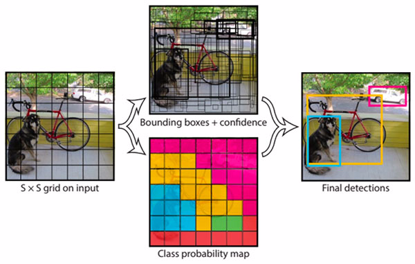
Figure 1: A simplified illustration of the YOLO object detector pipeline (source). We’ll use YOLO with OpenCV in this blog post.

When it comes to deep learning-based object detection, there are three primary object detectors you’ll encounter:

• R-CNN and their variants, including the original R-CNN, Fast R- CNN, and Faster R-CNN
• Single Shot Detector (SSDs)
• YOLO

R-CNNs are one of the first deep learning-based object detectors and are an example of a two-stage detector.

1. In the first R-CNN publication, Rich feature hierarchies for accurate object detection and semantic segmentation, (2013) Girshick et al. proposed an object detector that required an algorithm such as Selective Search (or equivalent) to propose candidate bounding boxes that could contain objects.
2. These regions were then passed into a CNN for classification, ultimately leading to one of the first deep learning-based object detectors.

The problem with the standard R-CNN method was that it was painfully slow and not a complete end-to-end object detector.

Girshick et al. published a second paper in 2015, entitled Fast R- CNN. The Fast R-CNN algorithm made considerable improvements to the original R-CNN, namely increasing accuracy and reducing the time it took to perform a forward pass; however, the model still relied on an external region proposal algorithm.

It wasn’t until Girshick et al.’s follow-up 2015 paper, Faster R-CNN: Towards Real-Time Object Detection with Region Proposal Networks, that R-CNNs became a true end-to-end deep learning object detector by removing the Selective Search requirement and instead relying on a Region Proposal Network (RPN) that is (1) fully convolutional and (2) can predict the object bounding boxes and “objectness” scores (i.e., a score quantifying how likely it is a region of an image may contain an image). The outputs of the RPNs are then passed into the R-CNN component for final classification and labeling.

While R-CNNs tend to very accurate, the biggest problem with the R-CNN family of networks is their speed — they were incredibly slow, obtaining only 5 FPS on a GPU.

To help increase the speed of deep learning-based object detectors, both Single Shot Detectors (SSDs) and YOLO use a one-stage detector strategy.

These algorithms treat object detection as a regression problem, taking a given input image and simultaneously learning bounding box coordinates and corresponding class label probabilities.

In general, single-stage detectors tend to be less accurate than two-stage detectors but are significantly faster.

YOLO is a great example of a single stage detector.

First introduced in 2015 by Redmon et al., their paper, You Only Look Once: Unified, Real-Time Object Detection, details an object detector capable of super real-time object detection, obtaining 45 FPS on a GPU.

Note: A smaller variant of their model called “Fast YOLO” claims to achieve 155 FPS on a GPU.

YOLO has gone through a number of different iterations, including YOLO9000: Better, Faster, Stronger (i.e., YOLOv2), capable of detecting over 9,000 object detectors.

Redmon and Farhadi are able to achieve such a large number of object detections by performing joint training for both object detection and classification. Using joint training the authors trained YOLO9000 simultaneously on both the ImageNet classification dataset and COCO detection dataset. The result is a YOLO model, called YOLO9000, that can predict detections for object classes that don’t have labeled detection data.

While interesting and novel, YOLOv2’s performance was a bit underwhelming given the title and abstract of the paper.

On the 156 class version of COCO, YOLO9000 achieved 16% mean Average Precision (mAP), and yes, while YOLO can detect 9,000 separate classes, the accuracy is not quite what we would desire.

Redmon and Farhadi recently published a new YOLO paper, YOLOv3: An Incremental Improvement (2018). YOLOv3 is significantly larger than previous models but is, in my opinion, the best one yet out of the YOLO family of object detectors.

We’ll be using YOLOv3 in this blog post, in particular, YOLO trained on the COCO dataset.

The COCO dataset consists of 80 labels, including, but not limited to:

• People
• Bicycles
• Cars and trucks
• Airplanes
• Stop signs and fire hydrants
• Animals, including cats, dogs, birds, horses, cows, and sheep, to name a few
• Kitchen and dining objects, such as wine glasses, cups, forks, knives, spoons, etc.
• …and much more!

You can find a full list of what YOLO trained on the COCO dataset can detect using this link.

I’ll wrap up this section by saying that any academic needs to read Redmon’s YOLO papers and tech reports — not only are they novel and insightful they are incredibly entertaining as well.

But seriously, if you do nothing else today read the YOLOv3 tech report.

It’s only 6 pages and one of those pages is just references/citations.

Furthermore, the tech report is honest in a way that academic papers rarely, if ever, are.

Project structure

Let’s take a look at today’s project layout. You can use your OS’s GUI (Finder for OSX, Nautilus for Ubuntu), but you may find it easier and faster to use the tree  command in your terminal:

$ tree
.
├── images
│   ├── baggage_claim.jpg
│   ├── dining_table.jpg
│   ├── living_room.jpg
│   └── soccer.jpg
├── output
│   ├── airport_output.avi
│   ├── car_chase_01_output.avi
│   ├── car_chase_02_output.avi
│   ├── car_chase_03_output.avi
│   └── overpass_output.avi
├── videos
│   ├── airport.mp4
│   ├── car_chase_01.mp4
│   ├── car_chase_02.mp4
│   ├── car_chase_03.mp4
│   └── overpass.mp4
├── yolo-coco
│   ├── coco.names
│   ├── yolov3.cfg
│   └── yolov3.weights
├── yolo.py
└── yolo_video.py
 
 directories,  files

Our project today consists of 4 directories and two Python scripts.

The directories (in order of importance) are:

• yolo-coco/ : The YOLOv3 object detector pre-trained (on the COCO dataset) model files. These were trained by the Darknet team.
• images/ : This folder contains four static images which we’ll perform object detection on for testing and evaluation purposes.
• videos/ : After performing object detection with YOLO on images, we’ll process videos in real time. This directory contains five sample videos for you to test with.
• output/ : Output videos that have been processed by YOLO and annotated with bounding boxes and class names can go in this folder.

We’re reviewing two Python scripts — yolo.py  and yolo_video.py . The first script is for images and then we’ll take what we learn and apply it to video in the second script.

Are you ready?

YOLO object detection in images

Let’s get started applying the YOLO object detector to images!

Open up the yolo.py  file in your project and insert the following code:

# import the necessary packages
import numpy as np
import argparse
import time
import cv2
import os
 
# construct the argument parse and parse the arguments
ap = argparse.ArgumentParser()
ap.add_argument("-i", "--image", required=True,
    help="path to input image")
ap.add_argument("-y", "--yolo", required=True,
    help="base path to YOLO directory")
ap.add_argument("-c", "--confidence", type=float, default=0.5,
    help="minimum probability to filter weak detections")
ap.add_argument("-t", "--threshold", type=float, default=0.3,
    help="threshold when applying non-maxima suppression")
args = vars(ap.parse_args())

All you need installed for this script OpenCV 3.4+ with Python bindings. You can find my OpenCV installation tutorials here, just keep in mind that OpenCV 4 is in beta right now — you may run into issues installing or running certain scripts since it’s not an official release. For the time being I recommend going for OpenCV 3.4+. You can actually be up and running in less than 5 minutes with pip as well.

First, we import our required packages — as long as OpenCV and NumPy are installed, your interpreter will breeze past these lines.

Now let’s parse four command line arguments. Command line arguments are processed at runtime and allow us to change the inputs to our script from the terminal. If you aren’t familiar with them, I encourage you to read more in my previous tutorial. Our command line arguments include:

• --image : The path to the input image. We’ll detect objects in this image using YOLO.
• --yolo : The base path to the YOLO directory. Our script will then load the required YOLO files in order to perform object detection on the image.
• --confidence : Minimum probability to filter weak detections. I’ve given this a default value of 50% ( 0.5 ), but you should feel free to experiment with this value.
• --threshold : This is our non-maxima suppression threshold with a default value of 0.3 . You can read more about non-maxima suppression here.

After parsing, the args  variable is now a dictionary containing the key-value pairs for the command line arguments. You’ll see args  a number of times in the rest of this script.

Let’s load our class labels and set random colors for each:

# load the COCO class labels our YOLO model was trained on
labelsPath = os.path.sep.join([args["yolo"], "coco.names"])
LABELS = open(labelsPath).read().strip().split("\n")
 
# initialize a list of colors to represent each possible class label
np.random.seed(42)
COLORS = np.random.randint(0, 255, size=(len(LABELS), 3),
    dtype="uint8")

Here we load all of our class LABELS  (notice the first command line argument, args["yolo"]  being used) on Lines 21 and 22. Random COLORS  are then assigned to each label on Lines 25-27.

Let’s derive the paths to the YOLO weights and configuration files followed by loading YOLO from disk:

# derive the paths to the YOLO weights and model configuration
weightsPath = os.path.sep.join([args["yolo"], "yolov3.weights"])
configPath = os.path.sep.join([args["yolo"], "yolov3.cfg"])
 
# load our YOLO object detector trained on COCO dataset (80 classes)
print("[INFO] loading YOLO from disk...")
net = cv2.dnn.readNetFromDarknet(configPath, weightsPath)

To load YOLO from disk on Line 35, we’ll take advantage of OpenCV’s DNN function calledcv2.dnn.readNetFromDarknet . This function requires both a configPath  and weightsPath  which are established via command line arguments on Lines 30 and 31.

I cannot stress this enough: you’ll need at least OpenCV 3.4 to run this code as it has the updated dnn  module required to load YOLO.

Let’s load the image and send it through the network:

# load our input image and grab its spatial dimensions
image = cv2.imread(args["image"])
(H, W) = image.shape[:2]
 
# determine only the *output* layer names that we need from YOLO
ln = net.getLayerNames()
ln = [ln[i[0] - 1] for i in net.getUnconnectedOutLayers()]
 
# construct a blob from the input image and then perform a forward
# pass of the YOLO object detector, giving us our bounding boxes and
# associated probabilities
blob = cv2.dnn.blobFromImage(image, 1 / 255.0, (416, 416),
    swapRB=True, crop=False)
net.setInput(blob)
start = time.time()
layerOutputs = net.forward(ln)
end = time.time()
 
# show timing information on YOLO
print("[INFO] YOLO took {:.6f} seconds".format(end - start))

 

In this block we:

• Load the input image  and extract its dimensions (Lines 38 and 39).
• Determine the output layer names from the YOLO model (Lines 42 and 43).
• Construct a blob  from the image (Lines 48 and 49). Are you confused about what a blob is or what the cv2.dnn.blobFromImage  does? Give this blog post a read.

Now that our blob is prepared, we’ll

• Perform a forward pass through our YOLO network (Lines 50 and 52)
• Show the inference time for YOLO (Line 56)

What good is object detection unless we visualize our results? Let’s take steps now to filter and visualize our results.

But first, let’s initialize some lists we’ll need in the process of doing so:

# initialize our lists of detected bounding boxes, confidences, and
# class IDs, respectively
boxes = []
confidences = []
classIDs = []

These lists include:

• boxes : Our bounding boxes around the object.
• confidences : The confidence value that YOLO assigns to an object. Lower confidence values indicate that the object might not be what the network thinks it is. Remember from our command line arguments above that we’ll filter out objects that don’t meet the 0.5  threshold.
• classIDs : The detected object’s class label.

Let’s begin populating these lists with data from our YOLO layerOutputs :

# loop over each of the layer outputs
for output in layerOutputs:
    # loop over each of the detections
    for detection in output:
        # extract the class ID and confidence (i.e., probability) of
        # the current object detection
        scores = detection[5:]
        classID = np.argmax(scores)
        confidence = scores[classID]
 
        # filter out weak predictions by ensuring the detected
        # probability is greater than the minimum probability
        if confidence > args["confidence"]:
            # scale the bounding box coordinates back relative to the
            # size of the image, keeping in mind that YOLO actually
            # returns the center (x, y)-coordinates of the bounding
            # box followed by the boxes' width and height
            box = detection[0:4] * np.array([W, H, W, H])
            (centerX, centerY, width, height) = box.astype("int")
 
            # use the center (x, y)-coordinates to derive the top and
            # and left corner of the bounding box
            x = int(centerX - (width / 2))
            y = int(centerY - (height / 2))
 
            # update our list of bounding box coordinates, confidences,
            # and class IDs
            boxes.append([x, y, int(width), int(height)])
            confidences.append(float(confidence))
            classIDs.append(classID)

 

There’s a lot here in this code block — let’s break it down.

In this block, we:

• Loop over each of the layerOutputs  (beginning on Line 65).
• Loop over each detection  in output  (a nested loop beginning on Line 67).
• Extract the classID  and confidence  (Lines 70-72).
• Use the confidence to filter out weak detections (Line 76).

Now that we’ve filtered out unwanted detections, we’re going to:

• Scale bounding box coordinates so we can display them properly on our original image (Line 81).
• Extract coordinates and dimensions of the bounding box (Line 82). YOLO returns bounding box coordinates in the form: (centerX, centerY, width, and height) .
• Use this information to derive the top-left (x, y)-coordinates of the bounding box (Lines 86 and 87).
• Update the boxes , confidences , and classIDs  lists (Lines 91-93).

With this data, we’re now going to apply what is called “non-maxima suppression”:

# apply non-maxima suppression to suppress weak, overlapping bounding
# boxes
idxs = cv2.dnn.NMSBoxes(boxes, confidences, args["confidence"],
    args["threshold"])

YOLO does not apply non-maxima suppression for us, so we need to explicitly apply it.

Applying non-maxima suppression suppresses significantly overlapping bounding boxes, keeping only the most confident ones.

NMS also ensures that we do not have any redundant or extraneous bounding boxes.

Taking advantage of OpenCV’s built-in DNN module implementation of NMS, we perform non-maxima suppression on Lines 97 and 98. All that is required is that we submit our boundingboxes , confidences , as well as both our confidence threshold and NMS threshold.

If you’ve been reading this blog, you might be wondering why we didn’t use my imutils implementation of NMS. The primary reason is that the NMSBoxes  function is now working in OpenCV. Previously it failed for some inputs and resulted in an error message. Now that theNMSBoxes  function is working, we can use it in our own scripts.

Let’s draw the boxes and class text on the image!

# ensure at least one detection exists
if len(idxs) > 0:
    # loop over the indexes we are keeping
    for i in idxs.flatten():
        # extract the bounding box coordinates
        (x, y) = (boxes[i][0], boxes[i][1])
        (w, h) = (boxes[i][2], boxes[i][3])
 
        # draw a bounding box rectangle and label on the image
        color = [int(c) for c in COLORS[classIDs[i]]]
        cv2.rectangle(image, (x, y), (x + w, y + h), color, 2)
        text = "{}: {:.4f}".format(LABELS[classIDs[i]], confidences[i])
        cv2.putText(image, text, (x, y - 5), cv2.FONT_HERSHEY_SIMPLEX,
            0.5, color, 2)
 
# show the output image
cv2.imshow("Image", image)
cv2.waitKey(0)

Assuming at least one detection exists (Line 101), we proceed to loop over idxs  determined by non-maxima suppression.

Then, we simply draw the bounding box and text on image  using our random class colors (Lines 105-113).

Finally, we display our resulting image until the user presses any key on their keyboard (ensuring the window opened by OpenCV is selected and focused).

---

To follow along with this guide, make sure you use the “Downloads” section of this tutorial to download the source code, YOLO model, and example images.

From there, open up a terminal and execute the following command:

$ python yolo.py --image images/baggage_claim.jpg --yolo yolo-coco
[INFO] loading YOLO from disk...
[INFO] YOLO took 0.347815 seconds

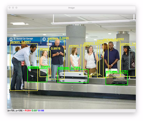
Figure 2: YOLO with OpenCV is used to detect people and baggage in an airport.

Here you can see that YOLO has not only detected each person in the input image, but also the suitcases as well!

Furthermore, if you take a look at the right corner of the image you’ll see that YOLO has also detected the handbag on the lady’s shoulder.

Let’s try another example:

$ python yolo.py --image images/living_room.jpg --yolo yolo-coco
[INFO] loading YOLO from disk...
[INFO] YOLO took 0.340221 seconds

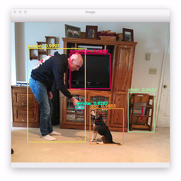
Figure 3: YOLO object detection with OpenCV is used to detect a person, dog, TV, and chair. The remote is a false-positive detection but looking at the ROI you could imagine that the area does share resemblances to a remote.

The image above contains a person (myself) and a dog (Jemma, the family beagle).

YOLO also detects the TV monitor and a chair as well. I’m particularly impressed that YOLO was able to detect the chair given that it’s handmade, old fashioned “baby high chair”.

Interestingly, YOLO thinks there is a “remote” in my hand. It’s actually not a remote — it’s the reflection of glass on a VHS tape; however, if you stare at the region it actually does look like it could be a remote.

The following example image demonstrates a limitation and weakness of the YOLO object detector:

$ python yolo.py --image images/dining_table.jpg --yolo yolo-coco
[INFO] loading YOLO from disk...
[INFO] YOLO took 0.362369 seconds

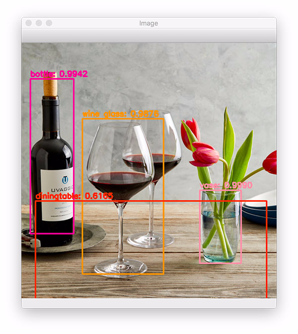
Figure 4: YOLO and OpenCV are used for object detection of a dining room table.

While both the wine bottle, dining table, and vase are correctly detected by YOLO, only one of the two wine glasses is properly detected.

We discuss why YOLO struggles with objects close together in the “Limitations and drawbacks of the YOLO object detector” section below.

Let’s try one final image:

$ python yolo.py --image images/soccer.jpg --yolo yolo-coco
[INFO] loading YOLO from disk...
[INFO] YOLO took 0.345656 seconds

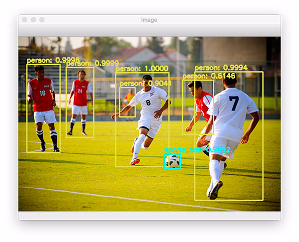
Figure 5: Soccer players and a soccer ball are detected with OpenCV using the YOLO object detector.

YOLO is able to correctly detect each of the players on the pitch, including the soccer ball itself. Notice the person in the background who is detected despite the area being highly blurred and partially obscured.

YOLO object detection in video streams

Now that we’ve learned how to apply the YOLO object detector to single images, let’s also utilize YOLO to perform object detection in input video files as well.

Open up the yolo_video.py  file and insert the following code:

# import the necessary packages
import numpy as np
import argparse
import imutils
import time
import cv2
import os
 
# construct the argument parse and parse the arguments
ap = argparse.ArgumentParser()
ap.add_argument("-i", "--input", required=True,
    help="path to input video")
ap.add_argument("-o", "--output", required=True,
    help="path to output video")
ap.add_argument("-y", "--yolo", required=True,
    help="base path to YOLO directory")
ap.add_argument("-c", "--confidence", type=float, default=0.5,
    help="minimum probability to filter weak detections")
ap.add_argument("-t", "--threshold", type=float, default=0.3,
    help="threshold when applyong non-maxima suppression")
args = vars(ap.parse_args())

We begin with our imports and command line arguments.

Notice that this script doesn’t have the --image  argument as before. To take its place, we now have two video-related arguments:

• --input : The path to the input video file.
• --output : Our path to the output video file.

Given these arguments, you can now use videos that you record of scenes with your smartphone or videos you find online. You can then process the video file producing an annotated output video. Of course if you want to use your webcam to process a live video stream, that is possible too. Just find examples on PyImageSearch where the  VideoStream  class from imutils.video  is utilized and make some minor changes.

Moving on, the next block is identical to the block from the YOLO image processing script:

# load the COCO class labels our YOLO model was trained on
labelsPath = os.path.sep.join([args["yolo"], "coco.names"])
LABELS = open(labelsPath).read().strip().split("\n")
 
# initialize a list of colors to represent each possible class label
np.random.seed(42)
COLORS = np.random.randint(0, 255, size=(len(LABELS), 3),
    dtype="uint8")
 
# derive the paths to the YOLO weights and model configuration
weightsPath = os.path.sep.join([args["yolo"], "yolov3.weights"])
configPath = os.path.sep.join([args["yolo"], "yolov3.cfg"])
 
# load our YOLO object detector trained on COCO dataset (80 classes)
# and determine only the *output* layer names that we need from YOLO
print("[INFO] loading YOLO from disk...")
net = cv2.dnn.readNetFromDarknet(configPath, weightsPath)
ln = net.getLayerNames()
ln = [ln[i[0] - 1] for i in net.getUnconnectedOutLayers()]

Here we load labels and generate colors followed by loading our YOLO model and determining output layer names.

Next, we’ll take care of some video-specific tasks:

# initialize the video stream, pointer to output video file, and
# frame dimensions
vs = cv2.VideoCapture(args["input"])
writer = None
(W, H) = (None, None)
 
# try to determine the total number of frames in the video file
try:
    prop = cv2.cv.CV_CAP_PROP_FRAME_COUNT if imutils.is_cv2() \
        else cv2.CAP_PROP_FRAME_COUNT
    total = int(vs.get(prop))
    print("[INFO] {} total frames in video".format(total))
 
# an error occurred while trying to determine the total
# number of frames in the video file
except:
    print("[INFO] could not determine # of frames in video")
    print("[INFO] no approx. completion time can be provided")
    total = -1

In this block, we:

• Open a file pointer to the video file for reading frames in the upcoming loop (Line 45).
• Initialize our video writer  and frame dimensions (Lines 46 and 47).
• Try to determine the total  number of frames in the video file so we can estimate how long processing the entire video will take (Lines 50-61).

Now we’re ready to start processing frames one by one:

# loop over frames from the video file stream
while True:
    # read the next frame from the file
    (grabbed, frame) = vs.read()
 
    # if the frame was not grabbed, then we have reached the end
    # of the stream
    if not grabbed:
        break
 
    # if the frame dimensions are empty, grab them
    if W is None or H is None:
        (H, W) = frame.shape[:2]

We define a while  loop (Line 64) and then we grab our first frame (Line 66).

We make a check to see if it is the last frame of the video. If so we need to break  from thewhile  loop (Lines 70 and 71).

Next, we grab the frame dimensions if they haven’t been grabbed yet (Lines 74 and 75).

Next, let’s perform a forward pass of YOLO, using our current frame  as the input:

    # construct a blob from the input frame and then perform a forward
    # pass of the YOLO object detector, giving us our bounding boxes
    # and associated probabilities
    blob = cv2.dnn.blobFromImage(frame, 1 / 255.0, (416, 416),
        swapRB=True, crop=False)
    net.setInput(blob)
    start = time.time()
    layerOutputs = net.forward(ln)
    end = time.time()
 
    # initialize our lists of detected bounding boxes, confidences,
    # and class IDs, respectively
    boxes = []
    confidences = []
    classIDs = []

Here we construct a blob  and pass it through the network, obtaining predictions. I’ve surrounded the forward pass operation with time stamps so we can calculate the elapsed time to make predictions on one frame — this will help us estimate the time needed to process the entire video.

We’ll then go ahead and initialize the same three lists we used in our previous script: boxes ,confidences , and classIDs .

This next block is, again, identical to our previous script:

    # loop over each of the layer outputs
    for output in layerOutputs:
        # loop over each of the detections
        for detection in output:
            # extract the class ID and confidence (i.e., probability)
            # of the current object detection
            scores = detection[5:]
            classID = np.argmax(scores)
            confidence = scores[classID]
 
            # filter out weak predictions by ensuring the detected
            # probability is greater than the minimum probability
            if confidence > args["confidence"]:
                # scale the bounding box coordinates back relative to
                # the size of the image, keeping in mind that YOLO
                # actually returns the center (x, y)-coordinates of
                # the bounding box followed by the boxes' width and
                # height
                box = detection[0:4] * np.array([W, H, W, H])
                (centerX, centerY, width, height) = box.astype("int")
 
                # use the center (x, y)-coordinates to derive the top
                # and and left corner of the bounding box
                x = int(centerX - (width / 2))
                y = int(centerY - (height / 2))
 
                # update our list of bounding box coordinates,
                # confidences, and class IDs
                boxes.append([x, y, int(width), int(height)])
                confidences.append(float(confidence))
                classIDs.append(classID)

In this code block, we:

• Loop over output layers and detections (Lines 94-96).
• Extract the classID  and filter out weak predictions (Lines 99-105).
• Compute bounding box coordinates (Lines 111-117).
• Update our respective lists (Lines 121-123).

Next, we’ll apply non-maxima suppression and begin to proceed to annotate the frame:

    # apply non-maxima suppression to suppress weak, overlapping
    # bounding boxes
    idxs = cv2.dnn.NMSBoxes(boxes, confidences, args["confidence"],
        args["threshold"])
 
    # ensure at least one detection exists
    if len(idxs) > 0:
        # loop over the indexes we are keeping
        for i in idxs.flatten():
            # extract the bounding box coordinates
            (x, y) = (boxes[i][0], boxes[i][1])
            (w, h) = (boxes[i][2], boxes[i][3])
 
            # draw a bounding box rectangle and label on the frame
            color = [int(c) for c in COLORS[classIDs[i]]]
            cv2.rectangle(frame, (x, y), (x + w, y + h), color, 2)
            text = "{}: {:.4f}".format(LABELS[classIDs[i]],
                confidences[i])
            cv2.putText(frame, text, (x, y - 5),
                cv2.FONT_HERSHEY_SIMPLEX, 0.5, color, 2)

You should recognize these lines as well. Here we:

• Apply NMS using the cv2.dnn.NMSBoxes  function (Lines 127 and 128) to suppress weak, overlapping bounding boxes. You can read more about non-maxima suppression here.
• Loop over the idxs  calculated by NMS and draw the corresponding bounding boxes + labels (Lines 131-144).

Let’s finish out the script:

    # check if the video writer is None
    if writer is None:
        # initialize our video writer
        fourcc = cv2.VideoWriter_fourcc(*"MJPG")
        writer = cv2.VideoWriter(args["output"], fourcc, 30,
            (frame.shape[1], frame.shape[0]), True)
 
        # some information on processing single frame
        if total > 0:
            elap = (end - start)
            print("[INFO] single frame took {:.4f} seconds".format(elap))
            print("[INFO] estimated total time to finish: {:.4f}".format(
                elap * total))
 
    # write the output frame to disk
    writer.write(frame)
 
# release the file pointers
print("[INFO] cleaning up...")
writer.release()
vs.release()

To wrap up, we simply:

• Initialize our video writer  if necessary (Lines 147-151). The writer  will be initialized on the first iteration of the loop.
• Print out our estimates of how long it will take to process the video (Lines 154-158).
• Write the frame  to the output video file (Line 161).
• Cleanup and release pointers (Lines 165 and 166).

---

To apply YOLO object detection to video streams, make sure you use the “Downloads” section of this blog post to download the source, YOLO object detector, and example videos.

From there, open up a terminal and execute the following command:

$ python yolo_video.py --input videos/car_chase_01.mp4 \
    --output output/car_chase_01.avi --yolo yolo-coco
[INFO] loading YOLO from disk...
[INFO]  total frames in video
[INFO] single frame took 0.3500 seconds
[INFO] estimated total time to finish: 204.0238
[INFO] cleaning up...

Figure 6: YOLO deep learning object detection applied to a car crash video.

Above you can see a GIF excerpt from a car chase video I found on YouTube.

In the video/GIF, you can see not only the vehicles being detected, but people, as well as the traffic lights, are detected too!

The YOLO object detector is performing quite well here. Let’s try a different video clip from the same car chase video:

$ python yolo_video.py --input videos/car_chase_02.mp4 \
    --output output/car_chase_02.avi --yolo yolo-coco
[INFO] loading YOLO from disk...
[INFO]  total frames in video
[INFO] single frame took 0.3455 seconds
[INFO] estimated total time to finish: 1082.0806
[INFO] cleaning up...

Figure 7: In this video of a suspect on the run, we have used OpenCV and YOLO object detection to find the person.

The suspect has now fled the car and is running across a parking lot.

YOLO is once again able to detect people.

At one point the suspect is actually able to make it back to their card and continue the chase — let’s see how YOLO performs there as well:

$ python yolo_video.py --input videos/car_chase_03.mp4 \
    --output output/car_chase_03.avi --yolo yolo-coco
[INFO] loading YOLO from disk...
[INFO]  total frames in video
[INFO] single frame took 0.3442 seconds
[INFO] estimated total time to finish: 257.8418
[INFO] cleaning up...

Figure 8: YOLO is a fast deep learning object detector capable of being used in real time video provided a GPU is utilized.

As a final example, let’s see how we may use YOLO as a starting point to building a traffic counter:

$ python yolo_video.py --input videos/overpass.mp4 \
    --output output/overpass.avi --yolo yolo-coco
[INFO] loading YOLO from disk...
[INFO]  total frames in video
[INFO] single frame took 0.3534 seconds
[INFO] estimated total time to finish: 286.9583
[INFO] cleaning up...

Figure 9: A video of traffic going under an overpass demonstrates that YOLO and OpenCV can be used to detect cars accurately and quickly.

I’ve put together a full video of YOLO object detection examples below:

Credits for video and audio:

• Car chase video posted on YouTube by Quaker Oats.
• Overpass video on YouTube by Vlad Kiraly.
• “White Crow” on the FreeMusicArchive by XTaKeRuX.

Limitations and drawbacks of the YOLO object detector

Arguably the largest limitation and drawback of the YOLO object detector is that:

1. It does not always handle small objects well
2. It especially does not handle objects grouped close together

The reason for this limitation is due to the YOLO algorithm itself:

• The YOLO object detector divides an input image into an SxS grid where each cell in the grid predicts only a single object.
• If there exist multiple, small objects in a single cell then YOLO will be unable to detect them, ultimately leading to missed object detections.

Therefore, if you know your dataset consists of many small objects grouped close together then you should not use the YOLO object detector.

In terms of small objects, Faster R-CNN tends to work the best; however, it’s also the slowest.

SSDs can also be used here; however, SSDs can also struggle with smaller objects (but not as much as YOLO).

SSDs often give a nice tradeoff in terms of speed and accuracy as well.

It’s also worth noting that YOLO ran slower than SSDs in this tutorial. In my previous tutorial on OpenCV object detection we utilized an SSD — a single forward pass of the SSD took ~0.03 seconds.

However, from this tutorial, we know that a forward pass of the YOLO object detector took ~0.3 seconds, approximately an order of magnitude slower!

If you’re using the pre-trained deep learning object detectors OpenCV supplies you may want to consider using SSDs over YOLO. From my personal experience, I’ve rarely encountered situations where I needed to use YOLO over SSDs:

• I have found SSDs much easier to train and their performance in terms of accuracy almost always outperforms YOLO (at least for the datasets I’ve worked with).
• YOLO may have excellent results on the COCO dataset; however, I have not found that same level of accuracy for my own tasks.

I, therefore, tend to use the following guidelines when picking an object detector for a given problem:

1. If I know I need to detect small objects and speed is not a concern, I tend to use Faster R-CNN.
2. If speed is absolutely paramount, I use YOLO.
3. If I need a middle ground, I tend to go with SSDs.

In most of my situations I end up using SSDs or RetinaNet — both are a great balance between the YOLO/Faster R-CNN.

Want to train your own deep learning object detectors?

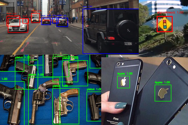
Figure 10: In my book, Deep Learning for Computer Vision with Python, I cover multiple object detection algorithms including Faster R-CNN, SSDs, and RetinaNet. Inside I will teach you how to create your object detection image dataset, train the object detector, and make predictions. Not to mention I also cover deep learning fundamentals, best practices, and my personal set of rules of thumb. Grab your copy now so you can start learning new skills.

The YOLO model we used in this tutorial was pre-trained on the COCO dataset…

…but what if you wanted to train a deep learning object detector on your own dataset?

Inside my book, Deep Learning for Computer Vision with Python, I’ll teach you how to train Faster R-CNNs, Single Shot Detectors (SSDs), and RetinaNet to:

• Detect logos in images
• Detect traffic signs (ex. stop sign, yield sign, etc.)
• Detect the front and rear views of vehicles (useful for building a self-driving car application)
• Detect weapons in images and video streams

All object detection chapters in the book include a detailed explanation of both the algorithm and code, ensuring you will be able to successfully train your own object detectors.

To learn more about my book (and grab your free set of sample chapters and table of contents), just click here.

Summary

In this tutorial we learned how to perform YOLO object detection using Deep Learning, OpenCV, and Python.

We then briefly discussed the YOLO architecture followed by implementing Python code to:

1. Apply YOLO object detection to single images
2. Apply the YOLO object detector to video streams

On my machine with a 3GHz Intel Xeon W processor, a single forward pass of YOLO took ~0.3 seconds; however, using a Single Shot Detector (SSD) from a previous tutorial, resulted in only 0.03 second detection, an order of magnitude faster!

For real-time deep learning-based object detection on your CPU with OpenCV and Python, you may want to consider using the SSD.

If you are interested in training your own deep learning object detectors on your own custom datasets, be sure to refer to my book, Deep Learning for Computer Vision with Python, where I provide detailed guides on how to successfully train your own detectors.

I hope you enjoyed today’s YOLO object detection tutorial!

来源： https://www.pyimagesearch.com/2018/11/12/yolo-object-detection-with-opencv/