利用tensorflow训练简单的生成对抗网络GAN

对抗网络是14年Goodfellow Ian在论文Generative Adversarial Nets中提出来的。 原理方面，对抗网络可以简单归纳为一个生成器(generator)和一个判断器(discriminator)之间博弈的过程。整个网络训练的过程中，

两个模块的分工

• 判断网络，直观来看就是一个简单的神经网络结构，输入就是一副图像，输出就是一个概率值，用于判断真假使用（概率值大于0.5那就是真，小于0.5那就是假）
• 生成网络，同样也可以看成是一个神经网络模型，输入是一组随机数Z，输出是一个图像。

两个模块的训练目的

• 判别网络的目的：就是能判别出来属于的一张图它是来自真实样本集还是假样本集。假如输入的是真样本，网络输出就接近1，输入的是假样本，网络输出接近0，那么很完美，达到了很好判别的目的。
• 生成网络的目的：生成网络是造样本的，它的目的就是使得自己造样本的能力尽可能强，强到判别网络没法判断是真样本还是假样本。

GAN的训练

　　需要注意的是生成模型与对抗模型可以说是完全独立的两个模型，好比就是完全独立的两个神经网络模型，他们之间没有什么联系。

那么训练这样的两个模型的大方法就是：单独交替迭代训练。因为是2个网络，不好一起训练，所以才去交替迭代训练，我们一一来看。

　　首先我们先随机产生一个生成网络模型（当然可能不是最好的生成网络），那么给一堆随机数组，就会得到一堆假的样本集（因为不是最终的生成模型，那么现在生成网络可能就处于劣势，导致生成的样本很糟糕，可能很容易就被判别网络判别出来了说这货是假冒的），但是先不管这个，假设我们现在有了这样的假样本集，真样本集一直都有，现在我们人为的定义真假样本集的标签，因为我们希望真样本集的输出尽可能为1，假样本集为0，很明显这里我们就已经默认真样本集所有的类标签都为1，而假样本集的所有类标签都为0.

　　对于生成网络，回想下我们的目标，是生成尽可能逼真的样本。那么原始的生成网络生成的样本你怎么知道它真不真呢？就是送到判别网络中，所以在训练生成网络的时候，我们需要联合判别网络一起才能达到训练的目的。就是如果我们单单只用生成网络，那么想想我们怎么去训练？误差来源在哪里？细想一下没有，但是如果我们把刚才的判别网络串接在生成网络的后面，这样我们就知道真假了，也就有了误差了。所以对于生成网络的训练其实是对生成-判别网络串接的训练，就像图中显示的那样。好了那么现在来分析一下样本，原始的噪声数组Z我们有，也就是生成了假样本我们有，此时很关键的一点来了，我们要把这些假样本的标签都设置为1，也就是认为这些假样本在生成网络训练的时候是真样本。这样才能起到迷惑判别器的目的，也才能使得生成的假样本逐渐逼近为正样本。

下面是代码部分，这里，我们利用训练的两个数据集分别是

• mnist
• Celeba

来生成手写数字以及人脸

首先是数据集的下载

 import math
 import os
 import hashlib
 from urllib.request import urlretrieve
 import zipfile
 import gzip
 import shutil
 
 data_dir = './data'
 
 def download_extract(database_name, data_path):
      """
      Download and extract database
      :param database_name: Database name
      """
      DATASET_CELEBA_NAME = 'celeba'
      DATASET_MNIST_NAME = 'mnist'
 
      if database_name == DATASET_CELEBA_NAME:
          url = 'https://s3-us-west-1.amazonaws.com/udacity-dlnfd/datasets/celeba.zip'
          hash_code = '00d2c5bc6d35e252742224ab0c1e8fcb'
          extract_path = os.path.join(data_path, 'img_align_celeba')
          save_path = os.path.join(data_path, 'celeba.zip')
          extract_fn = _unzip
      elif database_name == DATASET_MNIST_NAME:
          url = 'http://yann.lecun.com/exdb/mnist/train-images-idx3-ubyte.gz'
          hash_code = 'f68b3c2dcbeaaa9fbdd348bbdeb94873'
          extract_path = os.path.join(data_path, 'mnist')
          save_path = os.path.join(data_path, 'train-images-idx3-ubyte.gz')
          extract_fn = _ungzip
 
      if os.path.exists(extract_path):
          print('Found {} Data'.format(database_name))
          return
 
      if not os.path.exists(data_path):
          os.makedirs(data_path)
 
      if not os.path.exists(save_path):
          with DLProgress(unit='B', unit_scale=True, miniters=1, desc='Downloading {}'.format(database_name)) as pbar:
              urlretrieve(
                  url,
                  save_path,
                  pbar.hook)
 
      assert hashlib.md5(open(save_path, 'rb').read()).hexdigest() == hash_code, \
          '{} file is corrupted.  Remove the file and try again.'.format(save_path)
 
      os.makedirs(extract_path)
      try:
          extract_fn(save_path, extract_path, database_name, data_path)
      except Exception as err:
          shutil.rmtree(extract_path)  # Remove extraction folder if there is an error
          raise err
 
      # Remove compressed data
      os.remove(save_path)
 
 # download mnist
 download_extract('mnist', data_dir)
 # download celeba
 download_extract('celeba', data_dir

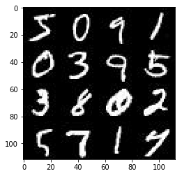
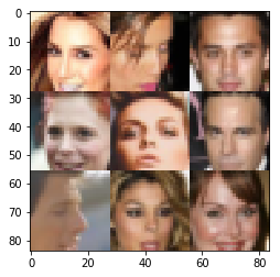
我们先看看我们的mnist还有celeba数据集是什么样子

 # the number of images
 show_n_images =16
 
 %matplotlib inline
 import os
 from glob import glob
 from matplotlib import pyplot
 
 def get_batch(image_files, width, height, mode):
     data_batch = np.array(
         [get_image(sample_file, width, height, mode) for sample_file in image_files]).astype(np.float32)
 
     # Make sure the images are in 4 dimensions
     if len(data_batch.shape) < 4:
         data_batch = data_batch.reshape(data_batch.shape + (1,))
 
     return data_batch
 
 def images_square_grid(images, mode):
     # Get maximum size for square grid of images
     save_size = math.floor(np.sqrt(images.shape[0]))
 
     # Scale to 0-255
     images = (((images - images.min()) * 255) / (images.max() - images.min())).astype(np.uint8)
 
     # Put images in a square arrangement
     images_in_square = np.reshape(
             images[:save_size*save_size],
             (save_size, save_size, images.shape[1], images.shape[2], images.shape[3]))
     if mode == 'L':
         images_in_square = np.squeeze(images_in_square, 4)
 
     # Combine images to grid image
     new_im = Image.new(mode, (images.shape[1] * save_size, images.shape[2] * save_size))
     for col_i, col_images in enumerate(images_in_square):
         for image_i, image in enumerate(col_images):
             im = Image.fromarray(image, mode)
             new_im.paste(im, (col_i * images.shape[1], image_i * images.shape[2]))
 
     return new_im
 
 mnist_images = get_batch(glob(os.path.join(data_dir, 'mnist/*.jpg'))[:show_n_images], 28, 28, 'L')
 pyplot.imshow(images_square_grid(mnist_images, 'L'), cmap='gray')

mninst：

 show_n_images = 9
 
 mnist_images = get_batch(glob(os.path.join(data_dir, 'img_align_celeba/*.jpg'))[:show_n_images], 28, 28, 'RGB')
 pyplot.imshow(images_square_grid(mnist_images, 'RGB'))

celeba

现在我们开始搭建网络

这里我建议用GPU来训练，tensorflow的版本最好是1.1.0

 from distutils.version import LooseVersion
 import warnings
 import tensorflow as tf
 
 # Check TensorFlow Version
 assert LooseVersion(tf.__version__) >= LooseVersion('1.0'), 'Please use TensorFlow version 1.0 or newer.  You are using {}'.format(tf.__version__)
 print('TensorFlow Version: {}'.format(tf.__version__))
 
 # Check for a GPU
 if not tf.test.gpu_device_name():
     warnings.warn('No GPU found. Please use a GPU to train your neural network.')
 else:
     print('Default GPU Device: {}'.format(tf.test.gpu_device_name()))

接着我们要做的是构建输入

 def model_inputs(image_width, image_height, image_channels, z_dim):
     ## Real imag
     inputs_real = tf.placeholder(tf.float32,(None, image_width,image_height,image_channels), name = 'input_real')
 
     ## input z
 
     inputs_z = tf.placeholder(tf.float32,(None, z_dim), name='input_z')
 
     ## Learning rate
     learning_rate = tf.placeholder(tf.float32, name = 'lr')
 
     return inputs_real, inputs_z, learning_rate

构建Discriminator

 def discriminator(images, reuse=False):
     """
     Create the discriminator network
     :param images: Tensor of input image(s)
     :param reuse: Boolean if the weights should be reused
     :return: Tuple of (tensor output of the discriminator, tensor logits of the discriminator)
     """
     # TODO: Implement Function
 
     ## scope here
 
     with tf.variable_scope('discriminator', reuse=reuse):
 
         alpha = 0.2  ### leak relu coeff
 
         # drop out probability
         keep_prob = 0.8
 
         # input layer 28 * 28 * color channel
         x1 = tf.layers.conv2d(images, 128, 5, strides=2, padding='same',
                               kernel_initializer= tf.contrib.layers.xavier_initializer(seed=2))
         ## No batch norm here
         ## leak relu here / alpha = 0.2
         relu1 = tf.maximum(alpha * x1, x1)
         # applied drop out here
         drop1 = tf.nn.dropout(relu1, keep_prob= keep_prob)
         # 14 * 14 * 128
 
         # Layer 2
         x2 = tf.layers.conv2d(drop1, 256, 5, strides=2, padding='same',
                              kernel_initializer= tf.contrib.layers.xavier_initializer(seed=2))
         ## employ batch norm here
         bn2 = tf.layers.batch_normalization(x2, training=True)
         ## leak relu
         relu2 = tf.maximum(alpha * bn2, bn2)
         drop2 = tf.nn.dropout(relu2, keep_prob=keep_prob)
 
         # 7 * 7 * 256 
 
         # Layer3
         x3 = tf.layers.conv2d(drop2, 512, 5, strides=2, padding='same',
                              kernel_initializer= tf.contrib.layers.xavier_initializer(seed=2))
         bn3 = tf.layers.batch_normalization(x3, training=True)
         relu3 = tf.maximum(alpha * bn3, bn3)
         drop3 = tf.nn.dropout(relu3, keep_prob=keep_prob)
         # 4 * 4 * 512
 
         # Output
         # Flatten
         flatten = tf.reshape(relu3, (-1, 4 * 4 * 512))
         logits = tf.layers.dense(flatten,1)
         # activation
         out = tf.nn.sigmoid(logits)
 
     return out, logits

接着是 Generator

 def generator(z, out_channel_dim, is_train=True):
     """
     Create the generator network
     :param z: Input z
     :param out_channel_dim: The number of channels in the output image
     :param is_train: Boolean if generator is being used for training
     :return: The tensor output of the generator
     """
     # TODO: Implement Function
 
     with tf.variable_scope('generator', reuse = not is_train):
         # First Fully connect layer
         x0 = tf.layers.dense(z, 4 * 4 * 512)
         # Reshape
         x0 = tf.reshape(x0,(-1,4,4,512))
         # Use the batch norm
         bn0 = tf.layers.batch_normalization(x0, training= is_train)
         # Leak relu
         relu0 = tf.nn.relu(bn0)
         # 4 * 4 * 512
 
         # Conv transpose here
         x1 = tf.layers.conv2d_transpose(relu0, 256, 4, strides=1, padding='valid')
         bn1 = tf.layers.batch_normalization(x1, training=is_train)
         relu1 = tf.nn.relu(bn1)
         # 7 * 7 * 256 
 
         x2 = tf.layers.conv2d_transpose(relu1, 128, 3, strides=2, padding='same')
         bn2 = tf.layers.batch_normalization(x2, training=is_train)
         relu2 = tf.nn.relu(bn2)
         # 14 * 14 * 128
 
         # Last cov
         logits = tf.layers.conv2d_transpose(relu2, out_channel_dim, 3, strides=2, padding='same')
         ## without batch norm here
         out = tf.tanh(logits)
 
         return out

然后我们来定义loss，这里，加入了smoother

 def model_loss(input_real, input_z, out_channel_dim):
     """
     Get the loss for the discriminator and generator
     :param input_real: Images from the real dataset
     :param input_z: Z input
     :param out_channel_dim: The number of channels in the output image
     :return: A tuple of (discriminator loss, generator loss)
     """
     # TODO: Implement Function
 
     g_model = generator(input_z, out_channel_dim, is_train=True)
 
     d_model_real, d_logits_real = discriminator(input_real, reuse = False)
 
     d_model_fake, d_logits_fake = discriminator(g_model, reuse= True)
 
     ## add smooth here
 
     smooth = 0.1
     d_loss_real = tf.reduce_mean(
         tf.nn.sigmoid_cross_entropy_with_logits(logits=d_logits_real,
                                                 labels=tf.ones_like(d_model_real) * (1 - smooth)))
 
     d_loss_fake = tf.reduce_mean(
         tf.nn.sigmoid_cross_entropy_with_logits(logits=d_logits_fake, labels=tf.zeros_like(d_model_fake)))
 
     g_loss = tf.reduce_mean(
         tf.nn.sigmoid_cross_entropy_with_logits(logits=d_logits_fake,
                                                 labels= tf.ones_like(d_model_fake)))
 
     d_loss = d_loss_real + d_loss_fake
 
     return d_loss, g_loss

接着我们需要定义网络优化的过程，这里我们需要用到batch_normlisation, 不懂的话去搜下文档

 def model_opt(d_loss, g_loss, learning_rate, beta1):
     """
     Get optimization operations
     :param d_loss: Discriminator loss Tensor
     :param g_loss: Generator loss Tensor
     :param learning_rate: Learning Rate Placeholder
     :param beta1: The exponential decay rate for the 1st moment in the optimizer
     :return: A tuple of (discriminator training operation, generator training operation)
     """
 
     t_vars = tf.trainable_variables()
     d_vars = [var for var in t_vars if var.name.startswith('discriminator')]
     g_vars = [var for var in t_vars if var.name.startswith('generator')] 
 
     update_ops = tf.get_collection(tf.GraphKeys.UPDATE_OPS)
 
     with tf.control_dependencies(update_ops):
         d_train_opt = tf.train.AdamOptimizer(learning_rate,beta1=beta1).minimize(d_loss,var_list = d_vars)
         g_train_opt = tf.train.AdamOptimizer(learning_rate,beta1=beta1).minimize(g_loss,var_list = g_vars)
 
     return d_train_opt, g_train_opt

现在，我们网络的模块，损失函数，以及优化的过程都定义好了，现在我们就要开始训练我们的网络了，我们的训练过程定义如下。

 def train(epoch_count, batch_size, z_dim, learning_rate, beta1, get_batches, data_shape, data_image_mode):
     """
     Train the GAN
     :param epoch_count: Number of epochs
     :param batch_size: Batch Size
     :param z_dim: Z dimension
     :param learning_rate: Learning Rate
     :param beta1: The exponential decay rate for the 1st moment in the optimizer
     :param get_batches: Function to get batches
     :param data_shape: Shape of the data
     :param data_image_mode: The image mode to use for images ("RGB" or "L")
     """
     losses = []
     samples = []
 
     input_real, input_z, lr = model_inputs(data_shape[1], data_shape[2], data_shape[3], z_dim)
 
     d_loss, g_loss = model_loss(input_real,input_z,data_shape[-1])
 
     d_opt, g_opt = model_opt(d_loss, g_loss, learning_rate, beta1)
 
     steps = 0
 
     with tf.Session() as sess:
         sess.run(tf.global_variables_initializer())
         for epoch_i in range(epoch_count):
             for batch_images in get_batches(batch_size):
                 # TODO: Train Model
                 steps += 1
 
                 # Reshape the image and pass to Discriminator
                 batch_images = batch_images.reshape(batch_size,
                                                     data_shape[1],
                                                     data_shape[2],
                                                     data_shape[3])
                 # Rescale the data to -1 and 1
                 batch_images = batch_images * 2
 
                 # Sample the noise
                 batch_z = np.random.uniform(-1,1,size = (batch_size, z_dim))
 
                 ## Run optimizer
                 _ = sess.run(d_opt, feed_dict = {input_real:batch_images,
                                                  input_z:batch_z,
                                                  lr:learning_rate
                                                  })
                 _ = sess.run(g_opt, feed_dict = {input_real:batch_images,
                                                  input_z:batch_z,
                                                  lr:learning_rate})
 
                 if steps % 10 == 0:
 
                     train_loss_d = d_loss.eval({input_real:batch_images, input_z:batch_z})
                     train_loss_g = g_loss.eval({input_real:batch_images, input_z:batch_z})
 
                     losses.append((train_loss_d,train_loss_g))
 
                     print("Epoch {}/{}...".format(epoch_i+1, epochs),
                           "Discriminator Loss: {:.4f}...".format(train_loss_d),
                           "Generator Loss: {:.4f}".format(train_loss_g))
 
                 if steps % 100 == 0:
 
                     show_generator_output(sess, 25, input_z, data_shape[-1], data_image_mode)

开始训练，超参数的设置

对于MNIST

 batch_size = 64
 z_dim = 100
 learning_rate = 0.001
 beta1 = 0.5
 epochs = 2
 
 mnist_dataset = helper.Dataset('mnist', glob(os.path.join(data_dir, 'mnist/*.jpg')))
 with tf.Graph().as_default():
     train(epochs, batch_size, z_dim, learning_rate, beta1, mnist_dataset.get_batches,
           mnist_dataset.shape, mnist_dataset.image_mode)

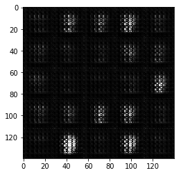
训练效果如下

开始的时候，网络的参数很差，我们生成的手写数字的效果自然就不好

随着训练的进行，轮廓逐渐清晰，效果如下，到最后：

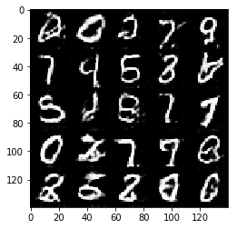
我们看到数字的轮廓基本是清晰可以辨认的，当然，这只是两个epoch的结果，如果有足够的时间经过更长时间的训练，效果会更好。

我们同样展示下对celeba人脸数据集的训练结果

 batch_size = 32
 z_dim = 100
 learning_rate = 0.001
 beta1 = 0.4
 epochs = 1
 
 celeba_dataset = helper.Dataset('celeba', glob(os.path.join(data_dir, 'img_align_celeba/*.jpg')))
 with tf.Graph().as_default():
     train(epochs, batch_size, z_dim, learning_rate, beta1, celeba_dataset.get_batches,
           celeba_dataset.shape, celeba_dataset.image_mode)

训练开始：

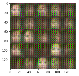
经过一个epoch之后：

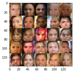
人脸的轮廓基本清晰了。

这里我们就是用了DCGAN最简单的方式来实现，原理过程说的不是很详细，同时，可能这个参数设置也不是很合理，训练的也不够成分，但是我想可以帮大家快速掌握实现一个简单的DCGAN的方法了。