CS231n 2016 通关 第三章-SVM 作业分析

作业内容，完成作业便可熟悉如下内容：

cell 1  设置绘图默认参数

 # Run some setup code for this notebook.
 
 import random
 import numpy as np
 from cs231n.data_utils import load_CIFAR10
 import matplotlib.pyplot as plt
 
 # This is a bit of magic to make matplotlib figures appear inline in the
 # notebook rather than in a new window.
 %matplotlib inline
 plt.rcParams['figure.figsize'] = (10.0, 8.0) # set default size of plots
 plt.rcParams['image.interpolation'] = 'nearest'
 plt.rcParams['image.cmap'] = 'gray'
 
 # Some more magic so that the notebook will reload external python modules;
 # see http://stackoverflow.com/questions/1907993/autoreload-of-modules-in-ipython
 %load_ext autoreload
 %autoreload 2

cell 2 读取数据得到数组（矩阵）

 # Load the raw CIFAR-10 data.
 cifar10_dir = 'cs231n/datasets/cifar-10-batches-py'
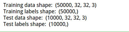
 X_train, y_train, X_test, y_test = load_CIFAR10(cifar10_dir)
 
 # As a sanity check, we print out the size of the training and test data.
 print 'Training data shape: ', X_train.shape
 print 'Training labels shape: ', y_train.shape
 print 'Test data shape: ', X_test.shape
 print 'Test labels shape: ', y_test.shape

得到结果，之后会用到，方便矩阵运算：

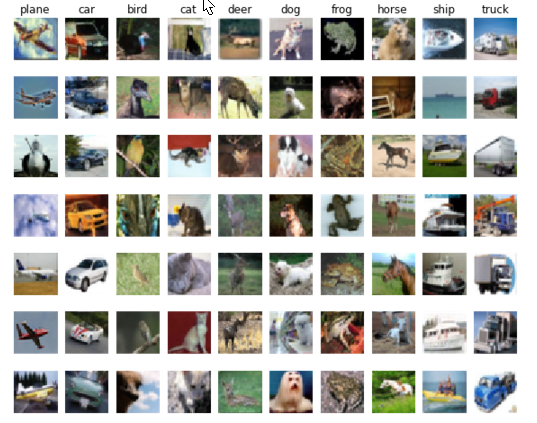
cell 3 对每一类随机选取对应的例子，并进行可视化：

 # Visualize some examples from the dataset.
 # We show a few examples of training images from each class.
 classes = ['plane', 'car', 'bird', 'cat', 'deer', 'dog', 'frog', 'horse', 'ship', 'truck']
 num_classes = len(classes)
 samples_per_class = 7
 for y, cls in enumerate(classes):
     idxs = np.flatnonzero(y_train == y)
     idxs = np.random.choice(idxs, samples_per_class, replace=False)
     for i, idx in enumerate(idxs):
         plt_idx = i * num_classes + y + 1
         plt.subplot(samples_per_class, num_classes, plt_idx)
         plt.imshow(X_train[idx].astype('uint8'))
         plt.axis('off')
         if i == 0:
             plt.title(cls)
 plt.show()

可视化结果：

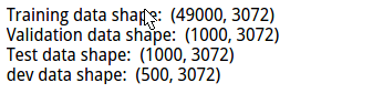
cell 4 将数据集划分为训练集，验证集。

 # Split the data into train, val, and test sets. In addition we will
 # create a small development set as a subset of the training data;
 # we can use this for development so our code runs faster.
 num_training = 49000
 num_validation = 1000
 num_test = 1000
 num_dev = 500
 
 # Our validation set will be num_validation points from the original
 # training set.
 mask = range(num_training, num_training + num_validation)
 X_val = X_train[mask]
 y_val = y_train[mask]
 
 # Our training set will be the first num_train points from the original
 # training set.
 mask = range(num_training)
 X_train = X_train[mask]
 y_train = y_train[mask]
 
 # We will also make a development set, which is a small subset of
 # the training set.
 mask = np.random.choice(num_training, num_dev, replace=False)
 X_dev = X_train[mask]
 y_dev = y_train[mask]
 
 # We use the first num_test points of the original test set as our
 # test set.
 mask = range(num_test)
 X_test = X_test[mask]
 y_test = y_test[mask]
 
 print 'Train data shape: ', X_train.shape
 print 'Train labels shape: ', y_train.shape
 print 'Validation data shape: ', X_val.shape
 print 'Validation labels shape: ', y_val.shape
 print 'Test data shape: ', X_test.shape
 print 'Test labels shape: ', y_test.shape

得到各个数据集的尺寸：

cell 5 将数据reshape，方便计算

 # Preprocessing: reshape the image data into rows
 X_train = np.reshape(X_train, (X_train.shape[0], -1))
 X_val = np.reshape(X_val, (X_val.shape[0], -1))
 X_test = np.reshape(X_test, (X_test.shape[0], -1))
 X_dev = np.reshape(X_dev, (X_dev.shape[0], -1))
 
 # As a sanity check, print out the shapes of the data
 print 'Training data shape: ', X_train.shape
 print 'Validation data shape: ', X_val.shape
 print 'Test data shape: ', X_test.shape
 print 'dev data shape: ', X_dev.shape

reshape 后的结果

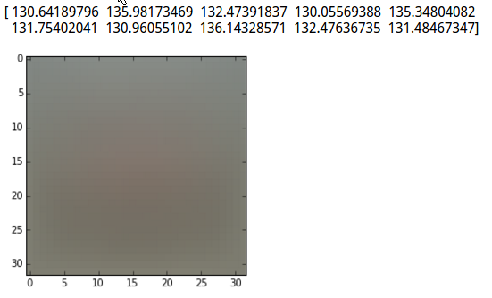
cell 6 计算训练集的均值

 # Preprocessing: subtract the mean image
 # first: compute the image mean based on the training data
 mean_image = np.mean(X_train, axis=0)
 print mean_image[:10] # print a few of the elements
 plt.figure(figsize=(4,4))
 plt.imshow(mean_image.reshape((32,32,3)).astype('uint8')) # visualize the mean image
 plt.show()

对均值可视化：

cell 7 训练集和测试集减去均值图像：

 # second: subtract the mean image from train and test data
 X_train -= mean_image
 X_val -= mean_image
 X_test -= mean_image
 X_dev -= mean_image

cell 8 将截距项b添加到数据里，方便计算

 # third: append the bias dimension of ones (i.e. bias trick) so that our SVM
 # only has to worry about optimizing a single weight matrix W.
 X_train = np.hstack([X_train, np.ones((X_train.shape[0], 1))])
 X_val = np.hstack([X_val, np.ones((X_val.shape[0], 1))])
 X_test = np.hstack([X_test, np.ones((X_test.shape[0], 1))])
 X_dev = np.hstack([X_dev, np.ones((X_dev.shape[0], 1))])
 
 print X_train.shape, X_val.shape, X_test.shape, X_dev.shape

数据尺寸：

此前步骤为初始步骤，基本不需要修改，之后是作业核心。

cell 9 使用for循环计算loss

 # Evaluate the naive implementation of the loss we provided for you:
 from cs231n.classifiers.linear_svm import svm_loss_naive
 import time
 
 # generate a random SVM weight matrix of small numbers
 W = np.random.randn(3073, 10) * 0.0001 
 
 loss, grad = svm_loss_naive(W, X_dev, y_dev, 0.00001)
 print 'loss: %f' % (loss, )

svm_loss_naive()具体实现：

 def svm_loss_naive(W, X, y, reg):
   """
   Structured SVM loss function, naive implementation (with loops).
 
   Inputs have dimension D, there are C classes, and we operate on minibatches
   of N examples.
 
   Inputs:
   - W: A numpy array of shape (D, C) containing weights.
   - X: A numpy array of shape (N, D) containing a minibatch of data.
   - y: A numpy array of shape (N,) containing training labels; y[i] = c means
     that X[i] has label c, where 0 <= c < C.
   - reg: (float) regularization strength
 
   Returns a tuple of:
   - loss as single float
   - gradient with respect to weights W; an array of same shape as W
   """
   dW = np.zeros(W.shape) # initialize the gradient as zero
 
   # compute the loss and the gradient
   # 10 classes
   num_classes = W.shape[1]
   #train 49000
   num_train = X.shape[0]
   loss = 0.0
   """
   for i ->49000:
     for j ->10:
         compute every train smaple about each class
   """
   #L = np.zeros(num_train,nun_class)
   for i in xrange(num_train):
     scores = X[i].dot(W)
     #1*3073 * 3073*10 >>1*10
     correct_class_score = scores[y[i]]
     for j in xrange(num_classes):
       if j == y[i]:
         continue
       margin = scores[j] - correct_class_score + 1 # note delta = 1
       if margin > 0:
         loss += margin
         #dW 3073*10
         dW[:,j] += X[i].T
         dW[:,y[i]] -= X[i].T
 
   # Right now the loss is a sum over all training examples, but we want it
   # to be an average instead so we divide by num_train.
   loss /= num_train
   dW /= num_train
   # Add regularization to the loss.
   # 1/2*w^2  w*w W*W = np.multiply(W,W)   >>>>elementwise product
   loss += reg * np.sum(W * W)
   dW +=reg*W
   #############################################################################
   # TODO:                                                                     #
   # Compute the gradient of the loss function and store it dW.                #
   # Rather that first computing the loss and then computing the derivative,   #
   # it may be simpler to compute the derivative at the same time that the     #
   # loss is being computed. As a result you may need to modify some of the    #
   # code above to compute the gradient.                                       #
   #############################################################################
   #computing coreect is differnt with others
   return loss, dW

loss结果为8.97460

cell 10 完善svm_loss_naive()，梯度下降更新变量：

 # Once you've implemented the gradient, recompute it with the code below
 # and gradient check it with the function we provided for you
 
 # Compute the loss and its gradient at W.
 loss, grad = svm_loss_naive(W, X_dev, y_dev, 0.0)
 
 # Numerically compute the gradient along several randomly chosen dimensions, and
 # compare them with your analytically computed gradient. The numbers should match
 # almost exactly along all dimensions.
 from cs231n.gradient_check import grad_check_sparse
 f = lambda w: svm_loss_naive(w, X_dev, y_dev, 0.0)[0]
 grad_numerical = grad_check_sparse(f, W, grad)
 
 # do the gradient check once again with regularization turned on
 # you didn't forget the regularization gradient did you?
 loss, grad = svm_loss_naive(W, X_dev, y_dev, 1e2)
 f = lambda w: svm_loss_naive(w, X_dev, y_dev, 1e2)[0]
 grad_numerical = grad_check_sparse(f, W, grad)

　　梯度更新代码已在cell9调用时给出。

梯度校验》》》使用解析法得到的dw与数值计算法得到的结果比较：

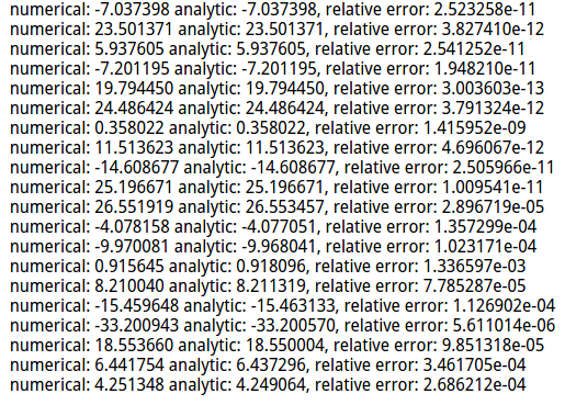
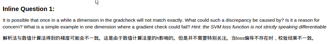
问题：

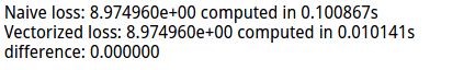
cell 11 使用向量（矩阵）的方式计算loss，并与之前的结果比较：

 # Next implement the function svm_loss_vectorized; for now only compute the loss;
 # we will implement the gradient in a moment.
 tic = time.time()
 loss_naive, grad_naive = svm_loss_naive(W, X_dev, y_dev, 0.00001)
 toc = time.time()
 print 'Naive loss: %e computed in %fs' % (loss_naive, toc - tic)
 
 from cs231n.classifiers.linear_svm import svm_loss_vectorized
 tic = time.time()
 loss_vectorized, _ = svm_loss_vectorized(W, X_dev, y_dev, 0.00001)
 toc = time.time()
 print 'Vectorized loss: %e computed in %fs' % (loss_vectorized, toc - tic)
 
 # The losses should match but your vectorized implementation should be much faster.
 print 'difference: %f' % (loss_naive - loss_vectorized)

差异结果：

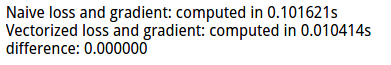
cell 12 使用向量（矩阵）的方式计算grad，并与之前的结果比较：

 # Complete the implementation of svm_loss_vectorized, and compute the gradient
 # of the loss function in a vectorized way.
 
 # The naive implementation and the vectorized implementation should match, but
 # the vectorized version should still be much faster.
 tic = time.time()
 _, grad_naive = svm_loss_naive(W, X_dev, y_dev, 0.00001)
 toc = time.time()
 print 'Naive loss and gradient: computed in %fs' % (toc - tic)
 
 tic = time.time()
 _, grad_vectorized = svm_loss_vectorized(W, X_dev, y_dev, 0.00001)
 toc = time.time()
 print 'Vectorized loss and gradient: computed in %fs' % (toc - tic)
 
 # The loss is a single number, so it is easy to compare the values computed
 # by the two implementations. The gradient on the other hand is a matrix, so
 # we use the Frobenius norm to compare them.
 difference = np.linalg.norm(grad_naive - grad_vectorized, ord='fro')
 print 'difference: %f' % difference

结果比较：

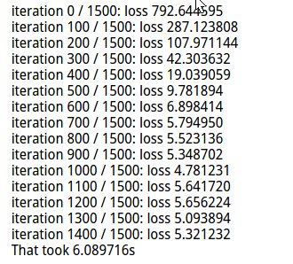
cell 13 随机梯度下降》》SGD

 # In the file linear_classifier.py, implement SGD in the function
 # LinearClassifier.train() and then run it with the code below.
 from cs231n.classifiers import LinearSVM
 svm = LinearSVM()
 tic = time.time()
 loss_hist = svm.train(X_train, y_train, learning_rate=1e-7, reg=5e4,
                       num_iters=1500, verbose=True)
 toc = time.time()
 print 'That took %fs' % (toc - tic)

loss 结果：

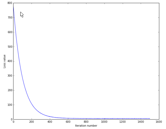
cell 14 画出loss变化曲线：

 # A useful debugging strategy is to plot the loss as a function of
 # iteration number:
 plt.plot(loss_hist)
 plt.xlabel('Iteration number')
 plt.ylabel('Loss value')
 plt.show()

结果：

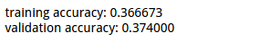
cell 15 用上述训练的参数，对验证集与训练集进行测试：

 # Write the LinearSVM.predict function and evaluate the performance on both the
 # training and validation set
 y_train_pred = svm.predict(X_train)
 print 'training accuracy: %f' % (np.mean(y_train == y_train_pred), )
 y_val_pred = svm.predict(X_val)
 print 'validation accuracy: %f' % (np.mean(y_val == y_val_pred), )

结果：

cell 16 对超参数》》学习率 正则化强度 使用训练集进行训练，使用验证集验证结果，选取最好的超参数。

 # Use the validation set to tune hyperparameters (regularization strength and
 # learning rate). You should experiment with different ranges for the learning
 # rates and regularization strengths; if you are careful you should be able to
 # get a classification accuracy of about 0.4 on the validation set.
 learning_rates = [1e-7, 2e-7, 3e-7, 5e-5, 8e-7]
 regularization_strengths = [1e4, 2e4, 3e4, 4e4, 5e4, 6e4, 7e4, 8e4, 1e5]
 
 # results is dictionary mapping tuples of the form
 # (learning_rate, regularization_strength) to tuples of the form
 # (training_accuracy, validation_accuracy). The accuracy is simply the fraction
 # of data points that are correctly classified.
 results = {}
 best_val = -1   # The highest validation accuracy that we have seen so far.
 best_svm = None # The LinearSVM object that achieved the highest validation rate.
 
 ################################################################################
 # TODO:                                                                        #
 # Write code that chooses the best hyperparameters by tuning on the validation #
 # set. For each combination of hyperparameters, train a linear SVM on the      #
 # training set, compute its accuracy on the training and validation sets, and  #
 # store these numbers in the results dictionary. In addition, store the best   #
 # validation accuracy in best_val and the LinearSVM object that achieves this  #
 # accuracy in best_svm.                                                        #
 #                                                                              #
 # Hint: You should use a small value for num_iters as you develop your         #
 # validation code so that the SVMs don't take much time to train; once you are #
 # confident that your validation code works, you should rerun the validation   #
 # code with a larger value for num_iters.                                      #
 ################################################################################
 iters = 1500
 for lr in learning_rates:
     for rs in regularization_strengths:
         svm = LinearSVM()
         svm.train(X_train, y_train, learning_rate=lr, reg=rs, num_iters=iters)
         y_train_pred = svm.predict(X_train)
         accu_train = np.mean(y_train == y_train_pred)
         y_val_pred = svm.predict(X_val)
         accu_val = np.mean(y_val == y_val_pred)
 
         results[(lr, rs)] = (accu_train, accu_val)
 
         if best_val < accu_val:
             best_val = accu_val
             best_svm = svm
 ################################################################################
 #                              END OF YOUR CODE                                #
 ################################################################################
 
 # Print out results.
 for lr, reg in sorted(results):
     train_accuracy, val_accuracy = results[(lr, reg)]
     print 'lr %e reg %e train accuracy: %f val accuracy: %f' % (
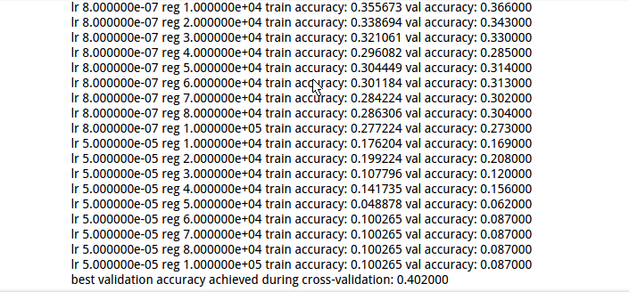
                 lr, reg, train_accuracy, val_accuracy)
 
 print 'best validation accuracy achieved during cross-validation: %f' % best_val

最终结果：

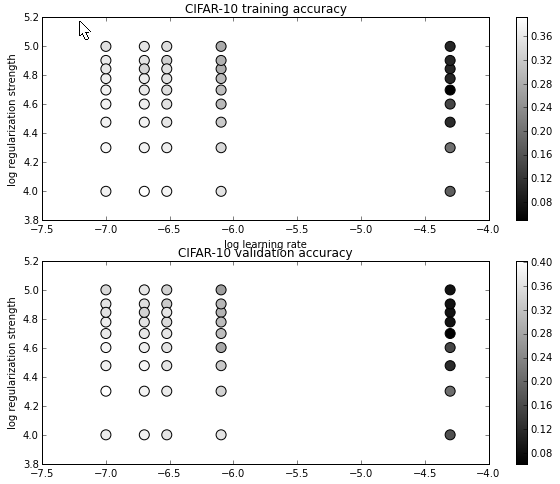
cell 17 对各组超参数的结果可视化：

 # Visualize the cross-validation results
 import math
 x_scatter = [math.log10(x[0]) for x in results]
 y_scatter = [math.log10(x[1]) for x in results]
 
 # plot training accuracy
 marker_size = 100
 colors = [results[x][0] for x in results]
 plt.subplot(2, 1, 1)
 plt.scatter(x_scatter, y_scatter, marker_size, c=colors)
 plt.colorbar()
 plt.xlabel('log learning rate')
 plt.ylabel('log regularization strength')
 plt.title('CIFAR-10 training accuracy')
 
 # plot validation accuracy
 colors = [results[x][1] for x in results] # default size of markers is 20
 plt.subplot(2, 1, 2)
 plt.scatter(x_scatter, y_scatter, marker_size, c=colors)
 plt.colorbar()
 plt.xlabel('log learning rate')
 plt.ylabel('log regularization strength')
 plt.title('CIFAR-10 validation accuracy')
 plt.show()

显示结果：

cell 18 使用得到最好超参数的模型对test集进行预测，比较预测值与真实值，计算准确率。

 # Evaluate the best svm on test set
 y_test_pred = best_svm.predict(X_test)
 test_accuracy = np.mean(y_test == y_test_pred)
 print 'linear SVM on raw pixels final test set accuracy: %f' % test_accuracy

结果：

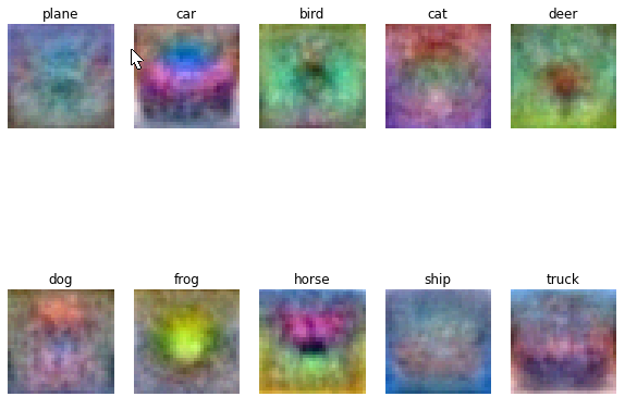
cell 19 对得到的w对应的class进行可视化：

 # Visualize the learned weights for each class.
 # Depending on your choice of learning rate and regularization strength, these may
 # or may not be nice to look at.
 w = best_svm.W[:-1,:] # strip out the bias
 w = w.reshape(32, 32, 3, 10)
 w_min, w_max = np.min(w), np.max(w)
 classes = ['plane', 'car', 'bird', 'cat', 'deer', 'dog', 'frog', 'horse', 'ship', 'truck']
 for i in xrange(10):
   plt.subplot(2, 5, i + 1)
 
   # Rescale the weights to be between 0 and 255
   wimg = 255.0 * (w[:, :, :, i].squeeze() - w_min) / (w_max - w_min)
   plt.imshow(wimg.astype('uint8'))
   plt.axis('off')
   plt.title(classes[i])

结果：

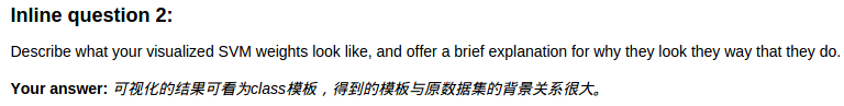
问题：

注：在softmax 与svm的超参数选择时，使用了共同的类，以及类中不同的相应的方法。具体的文件内容与注释如下。

附：通关CS231n企鹅群：578975100 validation：DL-CS231n