二、pandas入门
import numpy as np

import pandas as pd
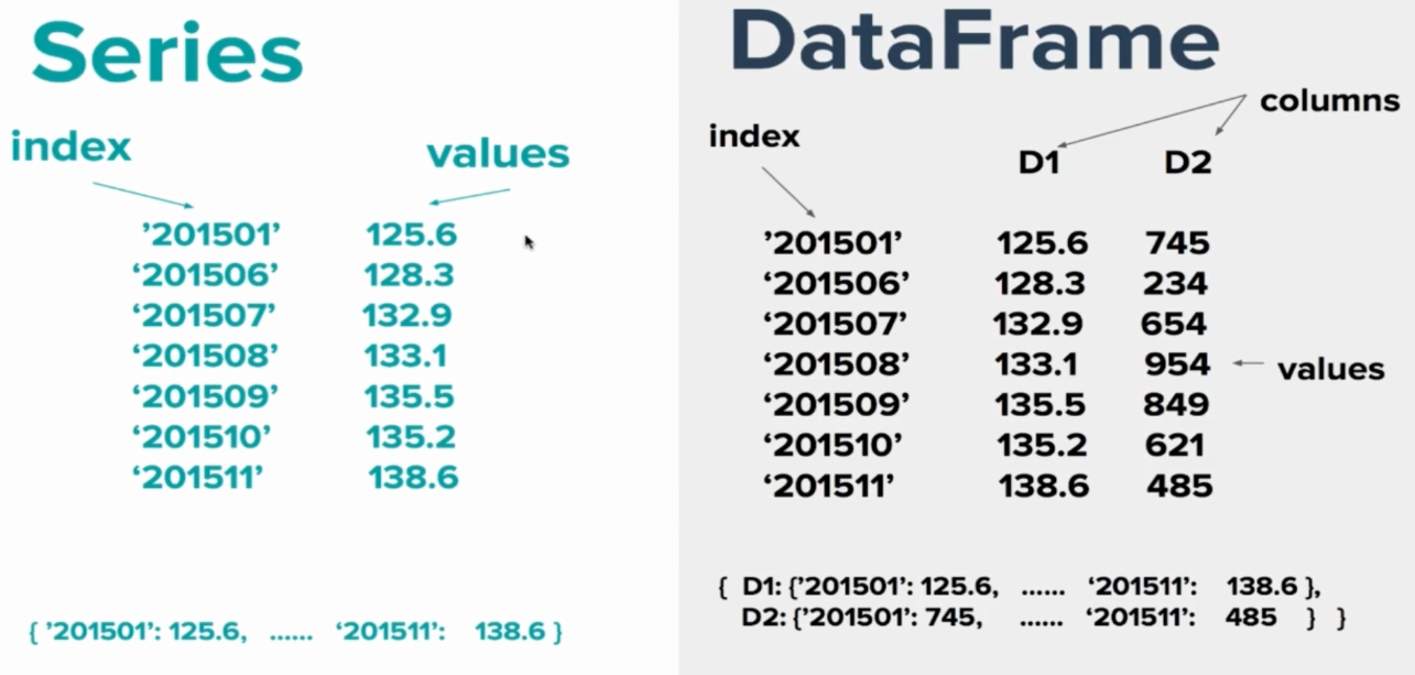
Series:
#创建Series方法1

s1=pd.Series([1,2,3,4])

s1
# 0    1

# 1    2

# 2    3

# 3    4

# dtype: int64
s1.values#array([1, 2, 3, 4], dtype=int64)

s1.index#RangeIndex(start=0, stop=4, step=1)
#创建Series方法2

s2=pd.Series(np.arange(5,10))

print(s2)
# 0    5

# 1    6

# 2    7

# 3    8

# 4    9

# dtype: int32
#创建Series方法3

s3=pd.Series({'5':1,'6':3,'7':9})

print(s3)
# 5    1

# 6    3

# 7    9

# dtype: int64
print(s3.index)#Index(['5', '6', '7'], dtype='object')
#创建Series方法4

s4=pd.Series([1,2,3,4],index=['A','B','C','D'])

print(s4)

# A    1

# B    2

# C    3

# D    4

# dtype: int64

#取值

print(s4['A'])#1

print(s4[s4>2])

# C    3

# D    4

# dtype: int64

#将Series转换成字典

dict=s4.to_dict()

print(dict)#{'A': 1, 'B': 2, 'C': 3, 'D': 4}

#将字典转换为Series

seri=pd.Series(dict)

print(seri)

# A    1

# B    2

# C    3

# D    4

# dtype: int64

#改变Series的index

index_1=['z','A','B','v','C']

s5=pd.Series(s4,index=index_1)

print(s5)

# z    NaN

# A    1.0

# B    2.0

# v    NaN

# C    3.0

# dtype: float64

#判断是不是null

print(pd.isnull(s5))

# z     True

# A    False

# B    False

# v     True

# C    False

# dtype: bool

print(pd.notnull(s5))

# z    False

# A     True

# B     True

# v    False

# C     True

# dtype: bool

#给Series起名字

s5.name='demo'

print(s5)

# z    NaN

# A    1.0

# B    2.0

# v    NaN

# C    3.0

# Name: demo, dtype: float64

s5.index.name='demo index'

print(s5.index)#Index(['z', 'A', 'B', 'v', 'C'], dtype='object', name='demo index')
DataFrame:
from pandas import Series,DataFrame

import webbrowser

link='https://www.tiobe.com/tiobe-index/'

webbrowser.open(link)#打开该网站

#复制网站中一下内容内容

'''

   Jan 2019  Jan 2018  Change Programming Language  Ratings Change.1

0         1         1     NaN                 Java  16.904%   +2.69%

1         2         2     NaN                    C  13.337%   +2.30%

2         3         4  change               Python   8.294%   +3.62%

3         4         3  change                  C++   8.158%   +2.55%

4         5         7  change    Visual Basic .NET   6.459%   +3.20%

'''

df=pd.read_clipboard()#从剪切板里创建DataFrame

type(df)#pandas.core.frame.DataFrame

print(df)#打印出和上述内容一样的DataFrame

#    Jan 2019  Jan 2018  Change Programming Language  Ratings Change.1

# 0         1         1     NaN                 Java  16.904%   +2.69%

# 1         2         2     NaN                    C  13.337%   +2.30%

# 2         3         4  change               Python   8.294%   +3.62%

# 3         4         3  change                  C++   8.158%   +2.55%

# 4         5         7  change    Visual Basic .NET   6.459%   +3.20%
#获取列名

print(df.columns)#Index(['Jan 2019', 'Jan 2018', 'Change', 'Programming Language', 'Ratings','Change.1'],dtype='object')
#获取某一列的value

print(df.Ratings)#获取Ratings列

# 0    16.904%

# 1    13.337%

# 2     8.294%

# 3     8.158%

# 4     6.459%

# Name: Ratings, dtype: object

print(df['Jan 2019'])#获取'Jan 2019'列,因为两个单词,所以不能用上式   获取两列则用print(df[['Jan 2019',Ratings]]),得到的类型为DataFrame

# 0    1

# 1    2

# 2    3

# 3    4

# 4    5

# Name: Jan 2019, dtype: int64

print(type(df.Ratings),type(df['Jan 2019']))#<class 'pandas.core.series.Series'> <class 'pandas.core.series.Series'>
# 提取旧的DataFrame某些列生成新的DataFrame

df_new=DataFrame(df,columns=['Programming Language','Jan 2019'])

print(df_new)

#   Programming Language  Jan 2019

# 0                 Java         1

# 1                    C         2

# 2               Python         3

# 3                  C++         4

# 4    Visual Basic .NET         5
#提取旧的DataFrame某些列生成新的DataFrame,但新的DataFrame中有的列在旧的没有,会生成新的列

df_new2=DataFrame(df,columns=['new lie','Jan 2019'])

print(df_new2)

#    new lie  Jan 2019

# 0      NaN         1

# 1      NaN         2

# 2      NaN         3

# 3      NaN         4

# 4      NaN         5

#可以给new lie赋值

df_new2['new lie']=range(5,10)

df_new2['new lie']=np.arange(5,10)#也可以通过numpy赋值

df_new2['new lie']=pd.Series(np.arange(5,10))#也可以通过Series赋值

print(df_new2)

#    new lie  Jan 2019

# 0        5         1

# 1        6         2

# 2        7         3

# 3        8         4

# 4        9         5

df_new2['new lie']=pd.Series([200,200],index=[2,3])#指定某一列某一两个元素值的更改

print(df_new2)

#    new lie  Jan 2019

# 0      NaN         1

# 1      NaN         2

# 2    200.0         3

# 3    200.0         4

# 4      NaN         5
Series与DataFrame:
import numpy as np

import pandas as pd

from pandas import Series,DataFrame

data={'country':['Belgium','India','Brazil'],

      'Capital':['Brussels','New Delhi','Brasillia'],

      'Population':[11190846,1303171035,207847528]}

#Seiries

s1=pd.Series(data['country'])

# 0    Belgium

# 1      India

# 2     Brazil

# dtype: object

s1.values#array(['Belgium', 'India', 'Brazil'], dtype=object)

s1.index#RangeIndex(start=0, stop=3, step=1)

#DataFrame

df1=pd.DataFrame(data)#通过字典创建DataFrame

# 	country	Capital	Population

# 0	Belgium	Brussels	11190846

# 1	India	New Delhi	1303171035

# 2	Brazil	Brasillia	207847528

df1['country']#访问某一列

df1.country##访问某一列的另一种方式,效果同上

# 0    Belgium

# 1      India

# 2     Brazil

# Name: country, dtype: object

type(df1['country'])#pandas.core.series.Series

#访问DataFrame的行

df1.iterrows()#<generator object DataFrame.iterrows at 0x0000000004E8F888>

for row in  df1.iterrows():

    print(row)

    print('类型:',type(row))

    print('长度:',len(row),'\n')

'''

(0, country        Belgium

Capital       Brussels

Population    11190846

Name: 0, dtype: object)

类型: <class 'tuple'>

长度: 2

(1, country            India

Capital        New Delhi

Population    1303171035

Name: 1, dtype: object)

类型: <class 'tuple'>

长度: 2

(2, country          Brazil

Capital       Brasillia

Population    207847528

Name: 2, dtype: object)

类型: <class 'tuple'>

长度: 2

'''

for row in  df1.iterrows():

    print('第一个:',row[0])

    print('第二个:', row[1],'\n')

    print('类型:',type(row[0]),type(row[1]))

    break

'''

第一个: 0

第二个: country        Belgium

Capital       Brussels

Population    11190846

Name: 0, dtype: object

类型: <class 'int'> <class 'pandas.core.series.Series'>

'''

#通过Series创建DataFrame

s1=pd.Series(data['Capital'])

s2=pd.Series(data['country'])

s3=pd.Series(data['Population'])

df_new1=pd.DataFrame([s1,s2,s3])

print(df_new1)

'''

          0           1          2

0  Brussels   New Delhi  Brasillia

1   Belgium       India     Brazil

2  11190846  1303171035  207847528

'''

print(df_new1.T)# 转置

'''

           0        1           2

0   Brussels  Belgium    11190846

1  New Delhi    India  1303171035

2  Brasillia   Brazil   207847528

'''

df_new2=pd.DataFrame([s1,s2,s3],index=['Capital','country','Population']).T

print(df_new2)

'''

     Capital  country  Population

0   Brussels  Belgium    11190846

1  New Delhi    India  1303171035

2  Brasillia   Brazil   207847528

'''
pandas中的DateFrame的IO操作:
import numpy as np

import pandas as pd

from pandas import Series,DataFrame

import webbrowser

link='http://pandas.pydata.org/pandas-docs/version/0.20/io.html'

webbrowser.open(link)#打开该网站

#复制网站中一下内容内容

'''

Format Type Data Description    Reader  Writer

text    CSV read_csv    to_csv

text    JSON    read_json   to_json

text    HTML    read_html   to_html

text    Local clipboard read_clipboard  to_clipboard

binary  MS Excel    read_excel  to_excel

binary  HDF5 Format read_hdf    to_hdf

binary  Feather Format  read_feather    to_feather

binary  Msgpack read_msgpack    to_msgpack

binary  Stata   read_stata  to_stata

binary  SAS read_sas

binary  Python Pickle Format    read_pickle to_pickle

SQL SQL read_sql    to_sql

SQL Google Big Query    read_gbq    to_gbq

'''

df1=pd.read_clipboard()

print(df1)

'''

   Format Type      Data Description          Reader        Writer

0         text                   CSV        read_csv        to_csv

1         text                  JSON       read_json       to_json

2         text                  HTML       read_html       to_html

3         text       Local clipboard  read_clipboard  to_clipboard

4       binary              MS Excel      read_excel      to_excel

5       binary           HDF5 Format        read_hdf        to_hdf

6       binary        Feather Format    read_feather    to_feather

7       binary               Msgpack    read_msgpack    to_msgpack

8       binary                 Stata      read_stata      to_stata

9       binary                   SAS        read_sas

10      binary  Python Pickle Format     read_pickle     to_pickle

11         SQL                   SQL        read_sql        to_sql

12         SQL      Google Big Query        read_gbq        to_gbq

'''

df1.to_clipboard()#将df1的内容复制到粘贴板

df1.to_csv('df1.csv')#将df1的内容输出到df1.csv文件中,包括index

df1.to_csv('df11.csv',index=False)#将df1的内容输出到df2.csv文件中,但不包括index

df2=pd.read_csv('df11.csv')#读取csv文件

print(df2)

'''

   Format Type      Data Description          Reader        Writer

0         text                   CSV        read_csv        to_csv

1         text                  JSON       read_json       to_json

2         text                  HTML       read_html       to_html

3         text       Local clipboard  read_clipboard  to_clipboard

4       binary              MS Excel      read_excel      to_excel

5       binary           HDF5 Format        read_hdf        to_hdf

6       binary        Feather Format    read_feather    to_feather

7       binary               Msgpack    read_msgpack    to_msgpack

8       binary                 Stata      read_stata      to_stata

9       binary                   SAS        read_sas

10      binary  Python Pickle Format     read_pickle     to_pickle

11         SQL                   SQL        read_sql        to_sql

12         SQL      Google Big Query        read_gbq        to_gbq

'''

df3=df1.to_json()#输出为json格式

print(df3)

'''

{"Format Type":{"0":"text","1":"text","2":"text","3":"text","4":"binary","5":"binary","6":"binary","7":"binary","8":"binary","9":"binary","10":"binary","11":"SQL","12":"SQL"},

"Data Description":{"0":"CSV","1":"JSON","2":"HTML","3":"Local clipboard","4":"MS Excel","5":"HDF5 Format","6":"Feather Format","7":"Msgpack","8":"Stata","9":"SAS","10":"Python Pickle Format","11":"SQL","12":"Google Big Query"},

"Reader":{"0":"read_csv","1":"read_json","2":"read_html","3":"read_clipboard","4":"read_excel","5":"read_hdf","6":"read_feather","7":"read_msgpack","8":"read_stata","9":"read_sas","10":"read_pickle","11":"read_sql","12":"read_gbq"},

"Writer":{"0":"to_csv","1":"to_json","2":"to_html","3":"to_clipboard","4":"to_excel","5":"to_hdf","6":"to_feather","7":"to_msgpack","8":"to_stata","9":" ","10":"to_pickle","11":"to_sql","12":"to_gbq"}}

'''

print(pd.read_json(df3))#读json格式

'''

   Format Type      Data Description          Reader        Writer

0         text                   CSV        read_csv        to_csv

1         text                  JSON       read_json       to_json

10      binary  Python Pickle Format     read_pickle     to_pickle

11         SQL                   SQL        read_sql        to_sql

12         SQL      Google Big Query        read_gbq        to_gbq

2         text                  HTML       read_html       to_html

3         text       Local clipboard  read_clipboard  to_clipboard

4       binary              MS Excel      read_excel      to_excel

5       binary           HDF5 Format        read_hdf        to_hdf

6       binary        Feather Format    read_feather    to_feather

7       binary               Msgpack    read_msgpack    to_msgpack

8       binary                 Stata      read_stata      to_stata

9       binary                   SAS        read_sas

'''

df1.to_json('df1.json')#生成json文件

print(pd.read_json('df1.json'))#读取json文件

'''

   Format Type      Data Description          Reader        Writer

0         text                   CSV        read_csv        to_csv

1         text                  JSON       read_json       to_json

10      binary  Python Pickle Format     read_pickle     to_pickle

11         SQL                   SQL        read_sql        to_sql

12         SQL      Google Big Query        read_gbq        to_gbq

2         text                  HTML       read_html       to_html

3         text       Local clipboard  read_clipboard  to_clipboard

4       binary              MS Excel      read_excel      to_excel

5       binary           HDF5 Format        read_hdf        to_hdf

6       binary        Feather Format    read_feather    to_feather

7       binary               Msgpack    read_msgpack    to_msgpack

8       binary                 Stata      read_stata      to_stata

9       binary                   SAS        read_sas

'''

df1.to_html('df1.html')#生成html文件

print(pd.read_html('df1.html'))#读取html文件

'''

[    Unnamed: 0 Format Type      Data Description          Reader        Writer

0            0        text                   CSV        read_csv        to_csv

1            1        text                  JSON       read_json       to_json

2            2        text                  HTML       read_html       to_html

3            3        text       Local clipboard  read_clipboard  to_clipboard

4            4      binary              MS Excel      read_excel      to_excel

5            5      binary           HDF5 Format        read_hdf        to_hdf

6            6      binary        Feather Format    read_feather    to_feather

7            7      binary               Msgpack    read_msgpack    to_msgpack

8            8      binary                 Stata      read_stata      to_stata

9            9      binary                   SAS        read_sas           NaN

10          10      binary  Python Pickle Format     read_pickle     to_pickle

11          11         SQL                   SQL        read_sql        to_sql

12          12         SQL      Google Big Query        read_gbq        to_gbq]

'''

df1.to_excel('df1.xlsx')#生成excell文件

print(pd.read_excel('df1.xlsx'))#读取excell文件

'''

   Format Type      Data Description          Reader        Writer

0         text                   CSV        read_csv        to_csv

1         text                  JSON       read_json       to_json

2         text                  HTML       read_html       to_html

3         text       Local clipboard  read_clipboard  to_clipboard

4       binary              MS Excel      read_excel      to_excel

5       binary           HDF5 Format        read_hdf        to_hdf

6       binary        Feather Format    read_feather    to_feather

7       binary               Msgpack    read_msgpack    to_msgpack

8       binary                 Stata      read_stata      to_stata

9       binary                   SAS        read_sas

10      binary  Python Pickle Format     read_pickle     to_pickle

11         SQL                   SQL        read_sql        to_sql

12         SQL      Google Big Query        read_gbq        to_gbq

'''
Series和DataFrame的indexing
import numpy as np

import pandas as pd

imdb=pd.read_csv(r'C:\Users\Administrator\Desktop\py_work\codes\presidential_polls.csv')

print(imdb.shape)#查看行列数   (10236, 27)

print(imdb.head())#默认打印前五行

'''

   cycle     branch        type                        matchup forecastdate  \

0   2016  President  polls-plus  Clinton vs. Trump vs. Johnson      11/1/16

1   2016  President  polls-plus  Clinton vs. Trump vs. Johnson      11/1/16

2   2016  President  polls-plus  Clinton vs. Trump vs. Johnson      11/1/16

3   2016  President  polls-plus  Clinton vs. Trump vs. Johnson      11/1/16

4   2016  President  polls-plus  Clinton vs. Trump vs. Johnson      11/1/16

      state   startdate     enddate                  pollster grade  \

0      U.S.  10/25/2016  10/31/2016   Google Consumer Surveys     B

1      U.S.  10/27/2016  10/30/2016  ABC News/Washington Post    A+

2  Virginia  10/27/2016  10/30/2016  ABC News/Washington Post    A+

3   Florida  10/20/2016  10/24/2016                 SurveyUSA     A

4      U.S.  10/20/2016  10/25/2016       Pew Research Center    B+

           ...           adjpoll_clinton adjpoll_trump  adjpoll_johnson  \

0          ...                  42.64140      40.86509         5.675099

1          ...                  43.29659      44.72984         3.401513

2          ...                  46.29779      40.72604         6.401513

3          ...                  46.35931      45.30585         1.777730

4          ...                  45.32744      42.20888         3.618320

   adjpoll_mcmullin  multiversions  \

0               NaN            NaN

1               NaN            NaN

2               NaN            NaN

3               NaN            NaN

4               NaN            NaN

                                                 url  poll_id  question_id  \

0  https://datastudio.google.com/u/0/#/org//repor...    47940        74999

1  http://www.langerresearch.com/wp-content/uploa...    47881        74936

2  https://www.washingtonpost.com/local/virginia-...    47880        74934

3  http://www.baynews9.com/content/news/baynews9/...    47465        74252

4  http://www.people-press.org/2016/10/27/as-elec...    47616        74519

   createddate             timestamp

0      11/1/16  15:09:38  1 Nov 2016

1      11/1/16  15:09:38  1 Nov 2016

2      11/1/16  15:09:38  1 Nov 2016

3     10/25/16  15:09:38  1 Nov 2016

4     10/27/16  15:09:38  1 Nov 2016

[5 rows x 27 columns]

'''

print(imdb.tail())#默认打印后5行,与head用法相同

'''

       cycle     branch        type                        matchup  \

10231   2016  President  polls-only  Clinton vs. Trump vs. Johnson

10232   2016  President  polls-only  Clinton vs. Trump vs. Johnson

10233   2016  President  polls-only  Clinton vs. Trump vs. Johnson

10234   2016  President  polls-only  Clinton vs. Trump vs. Johnson

10235   2016  President  polls-only  Clinton vs. Trump vs. Johnson

      forecastdate           state  startdate     enddate  \

10231      11/1/16         Alabama  9/30/2016  10/13/2016

10232      11/1/16        Virginia  9/30/2016   10/6/2016

10233      11/1/16        Virginia  9/16/2016   9/22/2016

10234      11/1/16  North Carolina  6/20/2016   6/21/2016

10235      11/1/16            Utah  7/29/2016   8/18/2016

                    pollster grade          ...           adjpoll_clinton  \

10231                  Ipsos    A-          ...                  37.30964

10232                  Ipsos    A-          ...                  49.13094

10233                  Ipsos    A-          ...                  45.97130

10234  Public Policy Polling    B+          ...                  45.29390

10235                  Ipsos    A-          ...                  31.62721

      adjpoll_trump  adjpoll_johnson  adjpoll_mcmullin  multiversions  \

10231      54.76821              NaN               NaN            NaN

10232      39.41588              NaN               NaN            NaN

10233      39.97518              NaN               NaN            NaN

10234      46.66175         1.596946               NaN            NaN

10235      44.65947              NaN               NaN            NaN

                                                     url  poll_id  \

10231              http://reuters.com/statesofthenation/    46817

10232          http://www.reuters.com/statesofthenation/    46675

10233          http://www.reuters.com/statesofthenation/    46096

10234  http://www.publicpolicypolling.com/pdf/2015/PP...    44400

10235           http://www.reuters.com/statesofthenation    44978

       question_id  createddate             timestamp

10231        73263     10/15/16  14:57:58  1 Nov 2016

10232        72969     10/10/16  14:57:58  1 Nov 2016

10233        72088      9/26/16  14:57:58  1 Nov 2016

10234        67363      6/23/16  14:57:58  1 Nov 2016

10235        69011      8/24/16  14:57:58  1 Nov 2016

[5 rows x 27 columns]

'''
print(imdb.iloc[10:13,0:5])#查看第10到12行,0到4列(iloc通过index搜索的,基于位置信息,类似切片,不包含末尾位置)

'''

    cycle     branch        type                        matchup forecastdate

10   2016  President  polls-plus  Clinton vs. Trump vs. Johnson      11/1/16

11   2016  President  polls-plus  Clinton vs. Trump vs. Johnson      11/1/16

12   2016  President  polls-plus  Clinton vs. Trump vs. Johnson      11/1/16

'''

df=imdb.iloc[10:13,0:5]

print(df.iloc[1:3,1:3])

'''

       branch        type

11  President  polls-plus

12  President  polls-plus

'''

print(df.loc[10:12,:'type'])#loc是通过lable查询的,基于lable信息查询,包含末尾位置

'''

    cycle     branch        type

10   2016  President  polls-plus

11   2016  President  polls-plus

12   2016  President  polls-plus

'''

print(imdb['adjpoll_clinton'].head())#查看某列

'''

0    42.64140

1    43.29659

2    46.29779

3    46.35931

4    45.32744

Name: adjpoll_clinton, dtype: float64

'''

print(imdb['adjpoll_clinton'][10])#查看某个元素  44.53217

print(imdb[['adjpoll_trump','adjpoll_johnson']])#通过某(些)列生成新的DataFrame

'''

       adjpoll_trump  adjpoll_johnson

0           40.86509         5.675099

1           44.72984         3.401513

2           40.72604         6.401513

3           45.30585         1.777730

4           42.20888         3.618320

5           42.26663         6.114222

6           43.56017         3.153590

7           43.50333         3.466432

8           37.24948         6.420006

9           41.69540         4.220173

10          43.84845              NaN

11          47.92262         2.676897

12          29.50605         3.170510

13          40.34972         5.823322

14          42.01937         6.499082

15          45.07725         3.499082

16          39.33826         5.044833

17          46.11255         3.054228

18          39.80679         6.359501

19          41.34735         4.421316

20          39.99571         6.272840

21          50.75720              NaN

22          38.87231         8.359501

23          41.55637         4.964521

24          43.84806         5.359501

25          45.03370         2.193952

26          44.78595         4.359501

27          44.18040         5.160502

28          40.41809         3.333669

29          49.47709         4.308866

...              ...              ...

10206       36.75014         9.152230

10207       40.08237              NaN

10208       43.67710              NaN

10209       43.40106              NaN

10210       35.52956              NaN

10211       35.03328              NaN

10212       44.77681              NaN

10213       38.24798              NaN

10214       41.25978              NaN

10215       41.59738              NaN

10216       41.64499         1.974752

10217       36.15054              NaN

10218       38.65057              NaN

10219       29.49314         9.007062

10220       37.87221              NaN

10221       39.42957              NaN

10222       53.95455              NaN

10223       33.07150         3.328916

10224       41.88533         1.974752

10225       36.82408         9.741756

10226       47.80848              NaN

10227       42.01089         3.671217

10228       45.06726              NaN

10229       40.16534        12.889780

10230       41.56030         2.872088

10231       54.76821              NaN

10232       39.41588              NaN

10233       39.97518              NaN

10234       46.66175         1.596946

10235       44.65947              NaN

[10236 rows x 2 columns]

'''
Series和DataFrame的Reindexing
import numpy as np

import pandas as pd

s1=pd.Series([1,2,3,4],index=['A','B','C','D'])

print(s1)
A    1

B    2

C    3

D    4

dtype: int64
print(s1.reindex(['A','C','E']))
A    1.0

C    3.0

E    NaN

dtype: float64
print(s1.reindex(['A','C','m'],fill_value=11))#通过fille_value填充数值
A     1

C     3

m    11

dtype: int64
s2=pd.Series(['a','b','c'],index=[1,5,10])

print(s2)
1     a

5     b

10    c

dtype: object
print(s2.reindex(index=range(15)))
0     NaN

1       a

2     NaN

3     NaN

4     NaN

5       b

6     NaN

7     NaN

8     NaN

9     NaN

10      c

11    NaN

12    NaN

13    NaN

14    NaN

dtype: object
print(s2.reindex(index=range(15),method='ffill'))#自动填充,第0个是NaN,第1到4用a填充(<=4),第5到9用b填充(大于等于5小于10),大于等于10用c填充
0     NaN

1       a

2       a

3       a

4       a

5       b

6       b

7       b

8       b

9       b

10      c

11      c

12      c

13      c

14      c

dtype: object
print(s2)
1     a

5     b

10    c

dtype: object
df1=pd.DataFrame(np.random.rand(25).reshape([5,5]))

print(df1)
          0         1         2         3         4

0  0.499115  0.244375  0.849224  0.348352  0.472657

1  0.676503  0.769790  0.479774  0.468003  0.703029

2  0.153982  0.699009  0.379184  0.151905  0.921860

3  0.904037  0.196925  0.421180  0.384442  0.642122

4  0.641124  0.748790  0.824351  0.101550  0.412564
df2=pd.DataFrame(np.random.rand(25).reshape([5,5]),index=['A','B','D','E','F'],columns=['c1','c2','c3','c4','c5'])

print(df2)
         c1        c2        c3        c4        c5

A  0.279563  0.267224  0.077868  0.080046  0.528182

B  0.660053  0.088954  0.512298  0.259552  0.108562

D  0.734865  0.776419  0.581695  0.578712  0.157753

E  0.926365  0.729410  0.328161  0.531319  0.550878

F  0.849754  0.770988  0.537104  0.833631  0.062303
print(df2.reindex(index=['A','B','C','D','E','F']))
         c1        c2        c3        c4        c5

A  0.279563  0.267224  0.077868  0.080046  0.528182

B  0.660053  0.088954  0.512298  0.259552  0.108562

C       NaN       NaN       NaN       NaN       NaN

D  0.734865  0.776419  0.581695  0.578712  0.157753

E  0.926365  0.729410  0.328161  0.531319  0.550878

F  0.849754  0.770988  0.537104  0.833631  0.062303
print(df2.reindex(columns=['c1','c2','c3','c4','c5','c6']))
         c1        c2        c3        c4        c5  c6

A  0.279563  0.267224  0.077868  0.080046  0.528182 NaN

B  0.660053  0.088954  0.512298  0.259552  0.108562 NaN

D  0.734865  0.776419  0.581695  0.578712  0.157753 NaN

E  0.926365  0.729410  0.328161  0.531319  0.550878 NaN

F  0.849754  0.770988  0.537104  0.833631  0.062303 NaN
print(df2.reindex(index=['A','B','C','D','E','F'],columns=['c1','c2','c3','c4','c5','c6']))
         c1        c2        c3        c4        c5  c6

A  0.279563  0.267224  0.077868  0.080046  0.528182 NaN

B  0.660053  0.088954  0.512298  0.259552  0.108562 NaN

C       NaN       NaN       NaN       NaN       NaN NaN

D  0.734865  0.776419  0.581695  0.578712  0.157753 NaN

E  0.926365  0.729410  0.328161  0.531319  0.550878 NaN

F  0.849754  0.770988  0.537104  0.833631  0.062303 NaN
s1=pd.Series([1,2,3,4],index=['A','B','C','D'])

print(s1)
A    1

B    2

C    3

D    4

dtype: int64
print(s1.reindex(['A','C']))#也可写成print(s1.reindex(index=['A','C']))
A    1

C    3

dtype: int64
print(df2.reindex(index=['A','C']))
         c1        c2        c3        c4        c5

A  0.279563  0.267224  0.077868  0.080046  0.528182

C       NaN       NaN       NaN       NaN       NaN
print(s1.drop(['B','C']))
A    1

D    4

dtype: int64
print(s1.drop('A'))
B    2

C    3

D    4

dtype: int64
print(df2.drop(['A'],axis=0))
         c1        c2        c3        c4        c5

B  0.660053  0.088954  0.512298  0.259552  0.108562

D  0.734865  0.776419  0.581695  0.578712  0.157753

E  0.926365  0.729410  0.328161  0.531319  0.550878

F  0.849754  0.770988  0.537104  0.833631  0.062303
print(df2.drop(['c1'],axis=1))
         c2        c3        c4        c5

A  0.267224  0.077868  0.080046  0.528182

B  0.088954  0.512298  0.259552  0.108562

D  0.776419  0.581695  0.578712  0.157753

E  0.729410  0.328161  0.531319  0.550878

F  0.770988  0.537104  0.833631  0.062303
谈一谈NaN-means Not a Number
n=np.nan

print(type(n))#<class 'float'>

print(1+n)#结果:nan   任何一个numuber与nan做运算结果永远都是not a nunmber
s1=pd.Series([1,2,np.nan,3,4],index=['A','B','C','D','E'])

print(s1)
A    1.0

B    2.0

C    NaN

D    3.0

E    4.0

dtype: float64
print(s1.isnull())
A    False

B    False

C     True

D    False

E    False

dtype: bool
View Cod
print(s1.notnull())
A     True

B     True

C    False

D     True

E     True

dtype: bool
print(s1.dropna())#drop掉value为nan的
A    1.0

B    2.0

D    3.0

E    4.0

dtype: float64
NaN in DataFrame
dframe=pd.DataFrame([[1,2,3],[np.nan,5,6],[7,np.nan,9],[np.nan,np.nan,np.nan]])

print(dframe)
     0    1    2

0  1.0  2.0  3.0

1  NaN  5.0  6.0

2  7.0  NaN  9.0

3  NaN  NaN  NaN
print(dframe.isnull())
       0      1      2

0  False  False  False

1   True  False  False

2  False   True  False

3   True   True   True
print(dframe.notnull())
       0      1      2

0   True   True   True

1  False   True   True

2   True  False   True

3  False  False  False
print(dframe.dropna())#默认axis=0,相当于print(dframe.dropna(axis=0)) 默认how='any'
     0    1    2

0  1.0  2.0  3.0
print(dframe.dropna(how='any'))#any指的是凡是含有nan的都会drop掉
     0    1    2

0  1.0  2.0  3.0
print(dframe.dropna(how='all'))#all指的是所有都是all的都会drop掉
     0    1    2

0  1.0  2.0  3.0

1  NaN  5.0  6.0

2  7.0  NaN  9.0
print(dframe.dropna(axis=1))#只剩下index了
Empty DataFrame

Columns: []

Index: [0, 1, 2, 3]
dframe2=pd.DataFrame([[1,2,3,np.nan],[2,np.nan,5,6],[np.nan,7,np.nan,9],[1,np.nan,np.nan,np.nan]])

print(dframe2)
     0    1    2    3

0  1.0  2.0  3.0  NaN

1  2.0  NaN  5.0  6.0

2  NaN  7.0  NaN  9.0

3  1.0  NaN  NaN  NaN
df2=dframe2.dropna()#默认thresh=None,相当于df2=dframe2.dropna(thresh=None)

print(df2)
Empty DataFrame

Columns: [0, 1, 2, 3]

Index: []
df3=dframe2.dropna(thresh=2)#只要一行中NaN个数大于2,就删除该行

print(df3)
     0    1    2    3

0  1.0  2.0  3.0  NaN

1  2.0  NaN  5.0  6.0

2  NaN  7.0  NaN  9.0
print(dframe2.fillna(value=10))#将NaN填充为10
      0     1     2     3

0   1.0   2.0   3.0  10.0

1   2.0  10.0   5.0   6.0

2  10.0   7.0  10.0   9.0

3   1.0  10.0  10.0  10.0
print(dframe2.fillna(value={0:'A',1:'16',2:'中国',3:'k'}))#将每列各自的NaN赋值,即:第0列用A填充,第1列用16填充。。。。。。

#注意:fillna和dropna不会改变原本的Series和DataFrame
   0   1   2  3

0  1   2   3  k

1  2  16   5  6

2  A   7  中国  9

3  1  16  中国  k
多级index
s1=pd.Series(np.random.rand(6),index=[['1','1','1','2','2','2'],['a','b','c','a','b','c']])

print(s1)
1  a    0.973831

   b    0.762415

   c    0.135763

2  a    0.974687

   b    0.471638

   c    0.573157

dtype: float64
print(type(s1))#<class 'pandas.core.series.Series'>
print(s1['1'])
a    0.973831

b    0.762415

c    0.135763

dtype: float64
print(type(s1['1']))#<class 'pandas.core.series.Series'>
print(s1['1']['a'])#0.9738309965219155
print(s1[:,'a'])
1    0.973831

2    0.974687

dtype: float64
#二级的series转换成dataframe(两种方法)

df1=s1.unstack()

print(df1)

df2=pd.DataFrame([s1['1'],s1['2']])

print(df2)
          a         b         c

1  0.973831  0.762415  0.135763

2  0.974687  0.471638  0.573157

          a         b         c

0  0.973831  0.762415  0.135763

1  0.974687  0.471638  0.573157
#dataframe转换成二级series

s2=df1.unstack()

print(s2)
a  1    0.973831

   2    0.974687

b  1    0.762415

   2    0.471638

c  1    0.135763

   2    0.573157

dtype: float64
print(df1.T.unstack())
1  a    0.973831

   b    0.762415

   c    0.135763

2  a    0.974687

   b    0.471638

   c    0.573157

dtype: float64
df=pd.DataFrame(np.arange(16).reshape(4,4),index=[['a','a','b','b'],[1,2,1,2]],columns=[['BJ','BJ','上海','广州'],[111,222,111,222]])

print(df)
     BJ      上海  广州

    111 222 111 222

a 1   0   1   2   3

  2   4   5   6   7

b 1   8   9  10  11

  2  12  13  14  15
print(df['BJ'])
     111  222

a 1    0    1

  2    4    5

b 1    8    9

  2   12   13
print(type(df['BJ']))#<class 'pandas.core.frame.DataFrame'>
print(df['BJ',111])#print(df['BJ'][111])效果相同
a  1     0

   2     4

b  1     8

   2    12

Name: (BJ, 111), dtype: int32
Mapping
df1=pd.DataFrame({'城市':['北京','上海','广州'],'人口':[1000,2000,1500]})

print(df1)
   城市    人口

0  北京  1000

1  上海  2000

2  广州  1500
#增加一列

df1['GDP']=pd.Series([9999,8888,7777])#方法一

print(df1)
   城市    人口   GDP

0  北京  1000  9999

1  上海  2000  8888

2  广州  1500  7777
salary={'北京':10,'上海':20,'广州':30}#方法二,尽量用此方法,原因看df2

df1['工资']=df1['城市'].map(salary)

print(df1)
   城市    人口   GDP  工资

0  北京  1000  9999  10

1  上海  2000  8888  20

2  广州  1500  7777  30
df2=pd.DataFrame({'城市':['北京','上海','广州'],'人口':[1000,2000,1500]},index=['A','B','C'])

print(df2)
   城市    人口

A  北京  1000

B  上海  2000

C  广州  1500
df2['GDP']=pd.Series([9999,8888,7777])

print(df2)
   城市    人口  GDP

A  北京  1000  NaN

B  上海  2000  NaN

C  广州  1500  NaN
df2['GGDDPP']=pd.Series([9999,8888,7777],index=['A','B','C'])

print(df2)
   城市    人口  GDP  GGDDPP

A  北京  1000  NaN    9999

B  上海  2000  NaN    8888

C  广州  1500  NaN    7777
Replace
s1=pd.Series(np.arange(100,105))

print(s1)
0    100

1    101

2    102

3    103

4    104

dtype: int32
print(s1.replace(101,np.nan))
0    100.0

1      NaN

2    102.0

3    103.0

4    104.0

dtype: float64
print(s1.replace({101:np.nan}))
0    100.0

1      NaN

2    102.0

3    103.0

4    104.0

dtype: float64
print(s1.replace([100,103,104],['中','eng','s']))
0      中

1    101

2    102

3    eng

4      s

dtype: object
print(s1)#s1并没有发生变化
0    100

1    101

2    102

3    103

4    104

dtype: int32
二、pandas入门的更多相关文章
- 利用Python进行数据分析——pandas入门
利用Python进行数据分析--pandas入门 基于NumPy建立的 from pandas importSeries,DataFrame,import pandas as pd 一.两种数据结构 ...
- 利用python进行数据分析之pandas入门
转自https://zhuanlan.zhihu.com/p/26100976 目录: 5.1 pandas 的数据结构介绍5.1.1 Series5.1.2 DataFrame5.1.3索引对象5. ...
- < 利用Python进行数据分析 - 第2版 > 第五章 pandas入门 读书笔记
<利用Python进行数据分析·第2版>第五章 pandas入门--基础对象.操作.规则 python引用.浅拷贝.深拷贝 / 视图.副本 视图=引用 副本=浅拷贝/深拷贝 浅拷贝/深拷贝 ...
- XML学习总结(二)——XML入门
XML学习总结(二)——XML入门 一.XML语法学习 学习XML语法的目的就是编写XML 一个XML文件分为如下几部分内容: 文档声明 元素 属性 注释 CDATA区 .特殊字符 处理指令(proc ...
- Spring+SpringMVC+MyBatis深入学习及搭建(十二)——SpringMVC入门程序(一)
转载请注明出处:http://www.cnblogs.com/Joanna-Yan/p/6999743.html 前面讲到:Spring+SpringMVC+MyBatis深入学习及搭建(十一)——S ...
- 基于tensorflow的MNIST手写数字识别(二)--入门篇
http://www.jianshu.com/p/4195577585e6 基于tensorflow的MNIST手写字识别(一)--白话卷积神经网络模型 基于tensorflow的MNIST手写数字识 ...
- 转:JAVAWEB开发之权限管理(二)——shiro入门详解以及使用方法、shiro认证与shiro授权
原文地址:JAVAWEB开发之权限管理(二)——shiro入门详解以及使用方法.shiro认证与shiro授权 以下是部分内容,具体见原文. shiro介绍 什么是shiro shiro是Apache ...
- Python 数据处理库 pandas 入门教程
Python 数据处理库 pandas 入门教程2018/04/17 · 工具与框架 · Pandas, Python 原文出处: 强波的技术博客 pandas是一个Python语言的软件包,在我们使 ...
- 深入浅出 JMS(二) - ActiveMQ 入门指南
深入浅出 JMS(二) - ActiveMQ 入门指南 上篇博文深入浅出 JMS(一) – JMS 基本概念,我们介绍了消息通信的规范JMS,这篇博文介绍一款开源的 JMS 具体实现-- Active ...
- 利用python进行数据分析--pandas入门2
随书练习,第五章 pandas入门2 # coding: utf-8 # In[1]: from pandas import Series,DataFrame import pandas as pd ...
随机推荐
- Flex Builder 装SVN
由于Flex Builder没有内置SVN支持,很是不便.为了方便,给Flex Builder也装了SVN插件.由于FB基于Eclipse,安装方法都是一样的. 选择 Help -> Soft ...
- 模拟定位工具gps mock
1. 到应用宝下载http://sj.qq.com/myapp/detail.htm?apkName=com.lexa.fakegps 2. 在 setting 里面 开发者选项 3. 把 模 ...
- 图数据库初探之Neo4j
图数据库初试之Neo4j 自从进入了移动互联网时代,各种新事物出现的速度都好像坐上了宇宙飞船,几乎隔几天一个新概念.就拿数据库而言,什么Oracle.DB2.SQL Server.MySQL,这些你都 ...
- 在junit格式的结果信息中只包含错误信息的修改方法
文件名称:suiteJunit.vm 文件路径:src\fitnesse\resources\templates 添加如下黑体部分内容: <?xml version="1.0" ...
- ZOJ3321,ZOJ3317
ZOJ3321 //there is at most one edge between two nodes. 因为这句话的局限性,又要满足环,那么一定是每个点度为2,然后为n节点的一个环 //#inc ...
- 原生js回到顶部
<!DOCTYPE html><html lang="en"><head> <meta charset="UTF-8" ...
- Xmind8 Pro 思维导图制作软件,傻瓜式安装激活教程
xmind 是做思维导图的软件?今天有一个以前的同事还在和我要这个软件,当然我支持正版啊 !因为正版好用! 我是一个不爱说废话的人,就顺便分享一下 给大家用! 软件下载地址: 链接:https://p ...
- iOS 7:漫谈#define 宏定义(转)
iOS :漫谈#define 宏定义 #define宏定义在C系开发中可以说占有举足轻重的作用.底层框架自不必说,为了编译优化和方便,以及跨平台能力,宏被大量使用,可以说底层开发离开define将寸步 ...
- Caffe实战五(Caffe可视化方法:编译matlab接口)
接上一篇文章,这里给出配置caffe后编译matlab接口的方法.(参考:<深度学习 21天实战Caffe 第16天 Caffe可视化方法>) 1.将Matlab目录更新至Caffe的Ma ...
- 115 Distinct Subsequences 不同子序列
给定一个字符串 S 和一个字符串 T,求 S 的不同的子序列中 T 出现的个数.一个字符串的一个子序列是指:通过删除一些(也可以不删除)字符且不干扰剩余字符相对位置所组成的新字符串.(譬如," ...