Python-根据成绩分析是否继续深造
案例:该数据集的是一个关于每个学生成绩的数据集,接下来我们对该数据集进行分析,判断学生是否适合继续深造
数据集特征展示
     GRE 成绩 (290 to 340)

     TOEFL 成绩(92 to 120)

     学校等级 (1 to 5)

     自身的意愿 (1 to 5)

     推荐信的力度 (1 to 5)

     CGPA成绩 (6.8 to 9.92)

     是否有研习经验 (0 or 1)

     读硕士的意向 (0.34 to 0.97)
1.导入包
import numpy as np

import pandas as pd

import matplotlib.pyplot as plt

import seaborn as sns

import os,sys
2.导入并查看数据集
df = pd.read_csv("D:\\machine-learning\\score\\Admission_Predict.csv",sep = ",")
print('There are ',len(df.columns),'columns')
for c in df.columns:
    sys.stdout.write(str(c)+', '
There are  9 columns

Serial No., GRE Score, TOEFL Score, University Rating, SOP, LOR , CGPA, Research, Chance of Admit ,
一共有9列特征
df.info()
<class 'pandas.core.frame.DataFrame'>

RangeIndex: 400 entries, 0 to 399

Data columns (total 9 columns):

Serial No.           400 non-null int64

GRE Score            400 non-null int64

TOEFL Score          400 non-null int64

University Rating    400 non-null int64

SOP                  400 non-null float64

LOR                  400 non-null float64

CGPA                 400 non-null float64

Research             400 non-null int64

Chance of Admit      400 non-null float64

dtypes: float64(4), int64(5)

memory usage: 28.2 KB

数据集信息:
  1.数据有9个特征,分别是学号,GRE分数,托福分数,学校等级,SOP,LOR,CGPA,是否参加研习,进修的几率
  2.数据集中没有空值
  3.一共有400条数据
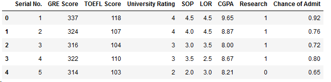
# 整理列名称

df = df.rename(columns={'Chance of Admit ':'Chance of Admit'})
# 显示前5列数据
df.head()
3.查看每个特征的相关性
fig,ax = plt.subplots(figsize=(10,10))

sns.heatmap(df.corr(),ax=ax,annot=True,linewidths=0.05,fmt='.2f',cmap='magma')

plt.show()
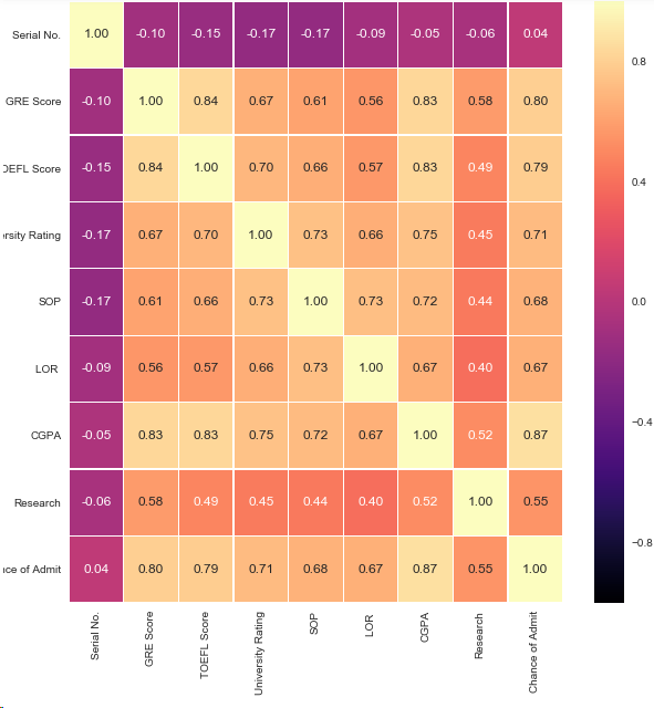
结论:1.最有可能影响是否读硕士的特征是GRE,CGPA,TOEFL成绩
2.影响相对较小的特征是LOR,SOP,和Research
4.数据可视化,双变量分析
4.1 进行Research的人数
print("Not Having Research:",len(df[df.Research == 0]))

print("Having Research:",len(df[df.Research == 1]))

y = np.array([len(df[df.Research == 0]),len(df[df.Research == 1])])

x = np.arange(2)

plt.bar(x,y)

plt.title("Research Experience")

plt.xlabel("Canditates")

plt.ylabel("Frequency")

plt.xticks(x,('Not having research','Having research'))

plt.show()
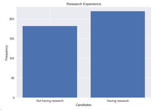
结论:进行research的人数是219,本科没有research人数是181
4.2 学生的托福成绩
y = np.array([df['TOEFL Score'].min(),df['TOEFL Score'].mean(),df['TOEFL Score'].max()])

x = np.arange(3)

plt.bar(x,y)

plt.title('TOEFL Score')

plt.xlabel('Level')

plt.ylabel('TOEFL Score')

plt.xticks(x,('Worst','Average','Best'))

plt.show()
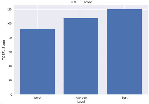
结论:最低分92分,最高分满分,进修学生的英语成绩很不错
4.3 GRE成绩
df['GRE Score'].plot(kind='hist',bins=200,figsize=(6,6))

plt.title('GRE Score')

plt.xlabel('GRE Score')

plt.ylabel('Frequency')

plt.show()
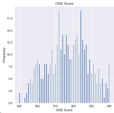
结论:310和330的分值的学生居多
4.4 CGPA和学校等级的关系
plt.scatter(df['University Rating'],df['CGPA'])

plt.title('CGPA Scores for University ratings')

plt.xlabel('University Rating')

plt.ylabel('CGPA')

plt.show()
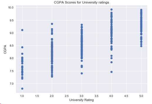
结论:学校越好,学生的GPA可能就越高
4.5 GRE成绩和CGPA的关系
plt.scatter(df['GRE Score'],df['CGPA'])

plt.title('CGPA for GRE Scores')

plt.xlabel('GRE Score')

plt.ylabel('CGPA')

plt.show()
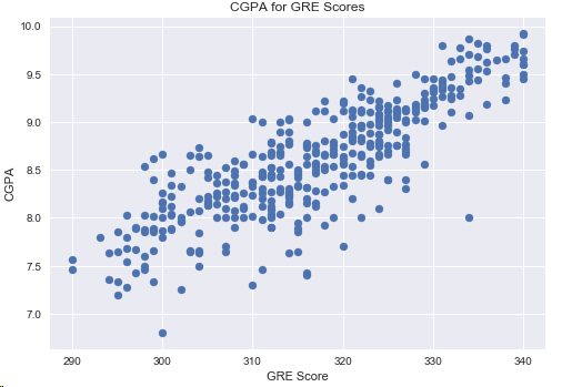
结论:GPA基点越高,GRE分数越高,2者的相关性很大
4.6 托福成绩和GRE成绩的关系
df[df['CGPA']>=8.5].plot(kind='scatter',x='GRE Score',y='TOEFL Score',color='red')

plt.xlabel('GRE Score')

plt.ylabel('TOEFL Score')

plt.title('CGPA >= 8.5')

plt.grid(True)

plt.show()

结论:多数情况下GRE和托福成正相关,但是GRE分数高,托福一定高。
4.6 学校等级和是否读硕士的关系
s = df[df['Chance of Admit'] >= 0.75]['University Rating'].value_counts().head(5)

plt.title('University Ratings of Candidates with an 75% acceptance chance')

s.plot(kind='bar',figsize=(20,10),cmap='Pastel1')

plt.xlabel('University Rating')

plt.ylabel('Candidates')

plt.show()

结论:排名靠前的学校的学生,进修的可能性更大
4.7 SOP和GPA的关系
plt.scatter(df['CGPA'],df['SOP'])

plt.xlabel('CGPA')

plt.ylabel('SOP')

plt.title('SOP for CGPA')

plt.show()
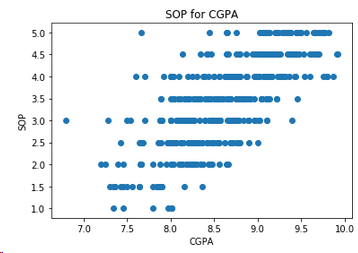
结论: GPA很高的学生,选择读硕士的自我意愿更强烈
4.8 SOP和GRE的关系
plt.scatter(df['GRE Score'],df['SOP'])

plt.xlabel('GRE Score')

plt.ylabel('SOP')

plt.title('SOP for GRE Score')

plt.show()
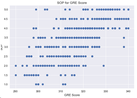
结论:读硕士意愿强的学生,GRE分数较高
5.模型
5.1 准备数据集
# 读取数据集

df = pd.read_csv('D:\\machine-learning\\score\\Admission_Predict.csv',sep=',')

serialNO = df['Serial No.'].values

df.drop(['Serial No.'],axis=1,inplace=True)

df = df.rename(columns={'Chance of Admit ':'Chance of Admit'})

# 分割数据集

y = df['Chance of Admit'].values

x = df.drop(['Chance of Admit'],axis=1)

from sklearn.model_selection import train_test_split

x_train,x_test,y_train,y_test = train_test_split(x,y,test_size=0.2,random_state=42)
# 归一化数据
from sklearn.preprocessing import MinMaxScaler
scaleX = MinMaxScaler(feature_range=[0,1])
x_train[x_train.columns] = scaleX.fit_transform(x_train[x_train.columns])
x_test[x_test.columns] = scaleX.fit_transform(x_test[x_test.columns])
5.2 回归
5.2.1 线性回归
from sklearn.linear_model import LinearRegression lr = LinearRegression()
lr.fit(x_train,y_train)
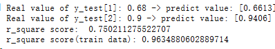
y_head_lr = lr.predict(x_test) print('Real value of y_test[1]: '+str(y_test[1]) + ' -> predict value: ' + str(lr.predict(x_test.iloc[[1],:])))
print('Real value of y_test[2]: '+str(y_test[2]) + ' -> predict value: ' + str(lr.predict(x_test.iloc[[2],:]))) from sklearn.metrics import r2_score
print('r_square score: ',r2_score(y_test,y_head_lr))
y_head_lr_train = lr.predict(x_train)
print('r_square score(train data):',r2_score(y_train,y_head_lr_train))

5.2.2 随机森林回归
from sklearn.ensemble import RandomForestRegressor

rfr = RandomForestRegressor(n_estimators=100,random_state=42)

rfr.fit(x_train,y_train)

y_head_rfr = rfr.predict(x_test)

print('Real value of y_test[1]: '+str(y_test[1]) + ' -> predict value: ' + str(rfr.predict(x_test.iloc[[1],:])))

print('Real value of y_test[2]: '+str(y_test[2]) + ' -> predict value: ' + str(rfr.predict(x_test.iloc[[2],:])))

from sklearn.metrics import r2_score

print('r_square score: ',r2_score(y_test,y_head_rfr))

y_head_rfr_train = rfr.predict(x_train)

print('r_square score(train data):',r2_score(y_train,y_head_rfr_train))
5.2.3 决策树回归
from sklearn.tree import DecisionTreeRegressor

dt = DecisionTreeRegressor(random_state=42)

dt.fit(x_train,y_train)

y_head_dt = dt.predict(x_test)

print('Real value of y_test[1]: '+str(y_test[1]) + ' -> predict value: ' + str(dt.predict(x_test.iloc[[1],:])))

print('Real value of y_test[2]: '+str(y_test[2]) + ' -> predict value: ' + str(dt.predict(x_test.iloc[[2],:])))

from sklearn.metrics import r2_score

print('r_square score: ',r2_score(y_test,y_head_dt))

y_head_dt_train = dt.predict(x_train)

print('r_square score(train data):',r2_score(y_train,y_head_dt_train))

5.2.4 三种回归方法比较
y = np.array([r2_score(y_test,y_head_lr),r2_score(y_test,y_head_rfr),r2_score(y_test,y_head_dt)])

x = np.arange(3)

plt.bar(x,y)

plt.title('Comparion of Regression Algorithms')

plt.xlabel('Regression')

plt.ylabel('r2_score')

plt.xticks(x,("LinearRegression","RandomForestReg.","DecisionTreeReg."))

plt.show()
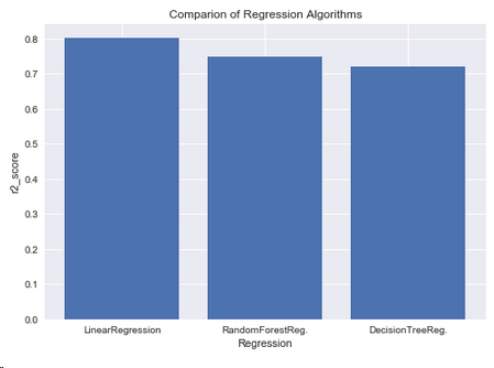
结论 : 回归算法中,线性回归的性能更优
5.2.5 三种回归方法与实际值的比较
red = plt.scatter(np.arange(0,80,5),y_head_lr[0:80:5],color='red')
blue = plt.scatter(np.arange(0,80,5),y_head_rfr[0:80:5],color='blue')
green = plt.scatter(np.arange(0,80,5),y_head_dt[0:80:5],color='green')
black = plt.scatter(np.arange(0,80,5),y_test[0:80:5],color='black')
plt.title('Comparison of Regression Algorithms')
plt.xlabel('Index of candidate')
plt.ylabel('Chance of admit')
plt.legend([red,blue,green,black],['LR','RFR','DT','REAL'])
plt.show()
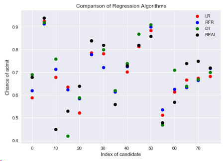
结论:在数据集中有70%的候选人有可能读硕士,从上图来看还有些点没有很好的得到预测
5.3 分类算法
5.3.1 准备数据
df = pd.read_csv('D:\\machine-learning\\score\\Admission_Predict.csv',sep=',')

SerialNO = df['Serial No.'].values

df.drop(['Serial No.'],axis=1,inplace=True)

df = df.rename(columns={'Chance of Admit ':'Chance of Admit'})

y = df['Chance of Admit'].values

x = df.drop(['Chance of Admit'],axis=1)

from sklearn.model_selection import train_test_split

x_train,x_test,y_train,y_test = train_test_split(x,y,test_size=0.2,random_state=42)

from sklearn.preprocessing import MinMaxScaler

scaleX = MinMaxScaler(feature_range=[0,1])

x_train[x_train.columns] = scaleX.fit_transform(x_train[x_train.columns])

x_test[x_test.columns] = scaleX.fit_transform(x_test[x_test.columns])

# 如果chance >0.8, chance of admit 就是1,否则就是0

y_train_01 = [1 if each > 0.8 else 0 for each in y_train]

y_test_01 = [1 if each > 0.8 else 0 for each in y_test]

y_train_01 = np.array(y_train_01)

y_test_01 = np.array(y_test_01)
5.3.2 逻辑回归
from sklearn.linear_model import LogisticRegression

lrc = LogisticRegression()

lrc.fit(x_train,y_train_01)

print('score: ',lrc.score(x_test,y_test_01))

print('Real value of y_test_01[1]: '+str(y_test_01[1]) + ' -> predict value: ' + str(lrc.predict(x_test.iloc[[1],:])))

print('Real value of y_test_01[2]: '+str(y_test_01[2]) + ' -> predict value: ' + str(lrc.predict(x_test.iloc[[2],:])))

from sklearn.metrics import confusion_matrix

cm_lrc = confusion_matrix(y_test_01,lrc.predict(x_test))

f,ax = plt.subplots(figsize=(5,5))

sns.heatmap(cm_lrc,annot=True,linewidths=0.5,linecolor='red',fmt='.0f',ax=ax)

plt.title('Test for Test dataset')

plt.xlabel('predicted y values')

plt.ylabel('real y value')

plt.show()

from sklearn.metrics import recall_score,precision_score,f1_score

print('precision_score is : ',precision_score(y_test_01,lrc.predict(x_test)))

print('recall_score is : ',recall_score(y_test_01,lrc.predict(x_test)))

print('f1_score is : ',f1_score(y_test_01,lrc.predict(x_test)))

# Test for Train Dataset:

cm_lrc_train = confusion_matrix(y_train_01,lrc.predict(x_train))

f,ax = plt.subplots(figsize=(5,5))

sns.heatmap(cm_lrc_train,annot=True,linewidths=0.5,linecolor='blue',fmt='.0f',ax=ax)

plt.title('Test for Train dataset')

plt.xlabel('predicted y values')

plt.ylabel('real y value')

plt.show()
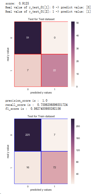
结论:1.通过混淆矩阵,逻辑回归算法在训练集样本上,有23个分错的样本,有72人想进一步读硕士
2.在测试集上有7个分错的样本
5.3.3 支持向量机(SVM)
from sklearn.svm import SVC

svm = SVC(random_state=1,kernel='rbf')

svm.fit(x_train,y_train_01)

print('score: ',svm.score(x_test,y_test_01))

print('Real value of y_test_01[1]: '+str(y_test_01[1]) + ' -> predict value: ' + str(svm.predict(x_test.iloc[[1],:])))

print('Real value of y_test_01[2]: '+str(y_test_01[2]) + ' -> predict value: ' + str(svm.predict(x_test.iloc[[2],:])))

from sklearn.metrics import confusion_matrix

cm_svm = confusion_matrix(y_test_01,svm.predict(x_test))

f,ax = plt.subplots(figsize=(5,5))

sns.heatmap(cm_svm,annot=True,linewidths=0.5,linecolor='red',fmt='.0f',ax=ax)

plt.title('Test for Test dataset')

plt.xlabel('predicted y values')

plt.ylabel('real y value')

plt.show()

from sklearn.metrics import recall_score,precision_score,f1_score

print('precision_score is : ',precision_score(y_test_01,svm.predict(x_test)))

print('recall_score is : ',recall_score(y_test_01,svm.predict(x_test)))

print('f1_score is : ',f1_score(y_test_01,svm.predict(x_test)))

# Test for Train Dataset:

cm_svm_train = confusion_matrix(y_train_01,svm.predict(x_train))

f,ax = plt.subplots(figsize=(5,5))

sns.heatmap(cm_svm_train,annot=True,linewidths=0.5,linecolor='blue',fmt='.0f',ax=ax)

plt.title('Test for Train dataset')

plt.xlabel('predicted y values')

plt.ylabel('real y value')

plt.show()
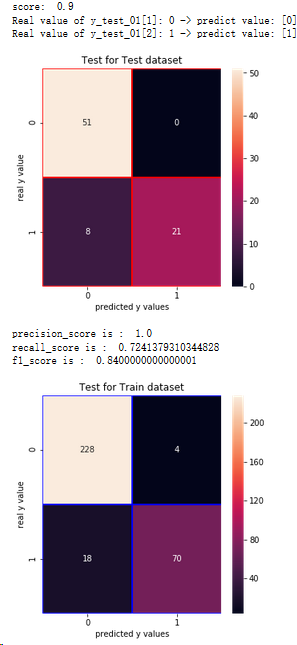
结论:1.通过混淆矩阵,SVM算法在训练集样本上,有22个分错的样本,有70人想进一步读硕士
2.在测试集上有8个分错的样本
5.3.4 朴素贝叶斯
from sklearn.naive_bayes import GaussianNB

nb = GaussianNB()

nb.fit(x_train,y_train_01)

print('score: ',nb.score(x_test,y_test_01))

print('Real value of y_test_01[1]: '+str(y_test_01[1]) + ' -> predict value: ' + str(nb.predict(x_test.iloc[[1],:])))

print('Real value of y_test_01[2]: '+str(y_test_01[2]) + ' -> predict value: ' + str(nb.predict(x_test.iloc[[2],:])))

from sklearn.metrics import confusion_matrix

cm_nb = confusion_matrix(y_test_01,nb.predict(x_test))

f,ax = plt.subplots(figsize=(5,5))

sns.heatmap(cm_nb,annot=True,linewidths=0.5,linecolor='red',fmt='.0f',ax=ax)

plt.title('Test for Test dataset')

plt.xlabel('predicted y values')

plt.ylabel('real y value')

plt.show()

from sklearn.metrics import recall_score,precision_score,f1_score

print('precision_score is : ',precision_score(y_test_01,nb.predict(x_test)))

print('recall_score is : ',recall_score(y_test_01,nb.predict(x_test)))

print('f1_score is : ',f1_score(y_test_01,nb.predict(x_test)))

# Test for Train Dataset:

cm_nb_train = confusion_matrix(y_train_01,nb.predict(x_train))

f,ax = plt.subplots(figsize=(5,5))

sns.heatmap(cm_nb_train,annot=True,linewidths=0.5,linecolor='blue',fmt='.0f',ax=ax)

plt.title('Test for Train dataset')

plt.xlabel('predicted y values')

plt.ylabel('real y value')

plt.show()
结论:1.通过混淆矩阵,朴素贝叶斯算法在训练集样本上,有20个分错的样本,有78人想进一步读硕士
2.在测试集上有7个分错的样本
5.3.5 随机森林分类器
from sklearn.ensemble import RandomForestClassifier

rfc = RandomForestClassifier(n_estimators=100,random_state=1)

rfc.fit(x_train,y_train_01)

print('score: ',rfc.score(x_test,y_test_01))

print('Real value of y_test_01[1]: '+str(y_test_01[1]) + ' -> predict value: ' + str(rfc.predict(x_test.iloc[[1],:])))

print('Real value of y_test_01[2]: '+str(y_test_01[2]) + ' -> predict value: ' + str(rfc.predict(x_test.iloc[[2],:])))

from sklearn.metrics import confusion_matrix

cm_rfc = confusion_matrix(y_test_01,rfc.predict(x_test))

f,ax = plt.subplots(figsize=(5,5))

sns.heatmap(cm_rfc,annot=True,linewidths=0.5,linecolor='red',fmt='.0f',ax=ax)

plt.title('Test for Test dataset')

plt.xlabel('predicted y values')

plt.ylabel('real y value')

plt.show()

from sklearn.metrics import recall_score,precision_score,f1_score

print('precision_score is : ',precision_score(y_test_01,rfc.predict(x_test)))

print('recall_score is : ',recall_score(y_test_01,rfc.predict(x_test)))

print('f1_score is : ',f1_score(y_test_01,rfc.predict(x_test)))

# Test for Train Dataset:

cm_rfc_train = confusion_matrix(y_train_01,rfc.predict(x_train))

f,ax = plt.subplots(figsize=(5,5))

sns.heatmap(cm_rfc_train,annot=True,linewidths=0.5,linecolor='blue',fmt='.0f',ax=ax)

plt.title('Test for Train dataset')

plt.xlabel('predicted y values')

plt.ylabel('real y value')

plt.show()

结论:1.通过混淆矩阵,随机森林算法在训练集样本上,有0个分错的样本,有88人想进一步读硕士
2.在测试集上有5个分错的样本
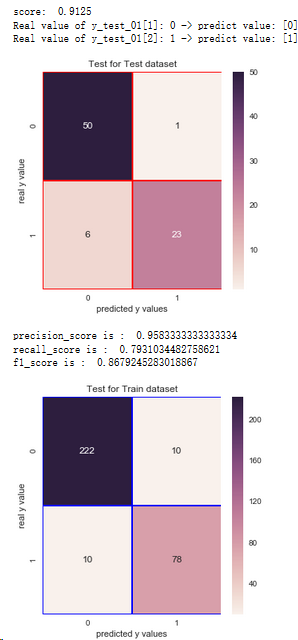
5.3.6 决策树分类器
from sklearn.tree import DecisionTreeClassifier

dtc = DecisionTreeClassifier(criterion='entropy',max_depth=3)

dtc.fit(x_train,y_train_01)

print('score: ',dtc.score(x_test,y_test_01))

print('Real value of y_test_01[1]: '+str(y_test_01[1]) + ' -> predict value: ' + str(dtc.predict(x_test.iloc[[1],:])))

print('Real value of y_test_01[2]: '+str(y_test_01[2]) + ' -> predict value: ' + str(dtc.predict(x_test.iloc[[2],:])))

from sklearn.metrics import confusion_matrix

cm_dtc = confusion_matrix(y_test_01,dtc.predict(x_test))

f,ax = plt.subplots(figsize=(5,5))

sns.heatmap(cm_dtc,annot=True,linewidths=0.5,linecolor='red',fmt='.0f',ax=ax)

plt.title('Test for Test dataset')

plt.xlabel('predicted y values')

plt.ylabel('real y value')

plt.show()

from sklearn.metrics import recall_score,precision_score,f1_score

print('precision_score is : ',precision_score(y_test_01,dtc.predict(x_test)))

print('recall_score is : ',recall_score(y_test_01,dtc.predict(x_test)))

print('f1_score is : ',f1_score(y_test_01,dtc.predict(x_test)))

# Test for Train Dataset:

cm_dtc_train = confusion_matrix(y_train_01,dtc.predict(x_train))

f,ax = plt.subplots(figsize=(5,5))

sns.heatmap(cm_dtc_train,annot=True,linewidths=0.5,linecolor='blue',fmt='.0f',ax=ax)

plt.title('Test for Train dataset')

plt.xlabel('predicted y values')

plt.ylabel('real y value')

plt.show()
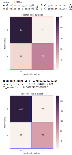
结论:1.通过混淆矩阵,决策树算法在训练集样本上,有20个分错的样本,有78人想进一步读硕士
2.在测试集上有7个分错的样本
5.3.7 K临近分类器
from sklearn.neighbors import KNeighborsClassifier

scores = []

for each in range(1,50):

    knn_n = KNeighborsClassifier(n_neighbors = each)

    knn_n.fit(x_train,y_train_01)

    scores.append(knn_n.score(x_test,y_test_01))

plt.plot(range(1,50),scores)

plt.xlabel('k')

plt.ylabel('Accuracy')

plt.show()

knn = KNeighborsClassifier(n_neighbors=7)

knn.fit(x_train,y_train_01)

print('score 7 : ',knn.score(x_test,y_test_01))

print('Real value of y_test_01[1]: '+str(y_test_01[1]) + ' -> predict value: ' + str(knn.predict(x_test.iloc[[1],:])))

print('Real value of y_test_01[2]: '+str(y_test_01[2]) + ' -> predict value: ' + str(knn.predict(x_test.iloc[[2],:])))

from sklearn.metrics import confusion_matrix

cm_knn = confusion_matrix(y_test_01,knn.predict(x_test))

f,ax = plt.subplots(figsize=(5,5))

sns.heatmap(cm_knn,annot=True,linewidths=0.5,linecolor='red',fmt='.0f',ax=ax)

plt.title('Test for Test dataset')

plt.xlabel('predicted y values')

plt.ylabel('real y value')

plt.show()

from sklearn.metrics import recall_score,precision_score,f1_score

print('precision_score is : ',precision_score(y_test_01,knn.predict(x_test)))

print('recall_score is : ',recall_score(y_test_01,knn.predict(x_test)))

print('f1_score is : ',f1_score(y_test_01,knn.predict(x_test)))

# Test for Train Dataset:

cm_knn_train = confusion_matrix(y_train_01,knn.predict(x_train))

f,ax = plt.subplots(figsize=(5,5))

sns.heatmap(cm_knn_train,annot=True,linewidths=0.5,linecolor='blue',fmt='.0f',ax=ax)

plt.title('Test for Train dataset')

plt.xlabel('predicted y values')

plt.ylabel('real y value')

plt.show()


结论:1.通过混淆矩阵,K临近算法在训练集样本上,有22个分错的样本,有71人想进一步读硕士
2.在测试集上有7个分错的样本
5.3.8 分类器比较
y = np.array([lrc.score(x_test,y_test_01),svm.score(x_test,y_test_01),nb.score(x_test,y_test_01),

              dtc.score(x_test,y_test_01),rfc.score(x_test,y_test_01),knn.score(x_test,y_test_01)])

x = np.arange(6)

plt.bar(x,y)

plt.title('Comparison of Classification Algorithms')

plt.xlabel('Classification')

plt.ylabel('Score')

plt.xticks(x,("LogisticReg.","SVM","GNB","Dec.Tree","Ran.Forest","KNN"))

plt.show()

结论:随机森林和朴素贝叶斯二者的预测值都比较高
5.4 聚类算法
5.4.1 准备数据
df = pd.read_csv('D:\\machine-learning\\score\\Admission_Predict.csv',sep=',')

df = df.rename(columns={'Chance of Admit ':'Chance of Admit'})

serialNo = df['Serial No.']

df.drop(['Serial No.'],axis=1,inplace=True)

df = (df - np.min(df)) / (np.max(df)-np.min(df))

y = df['Chance of Admit']

x = df.drop(['Chance of Admit'],axis=1)
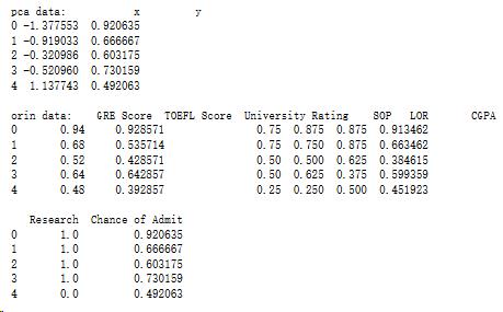
5.4.2 降维
from sklearn.decomposition import PCA

pca = PCA(n_components=1,whiten=True)

pca.fit(x)

x_pca = pca.transform(x)

x_pca = x_pca.reshape(400)

dictionary = {'x':x_pca,'y':y}

data = pd.DataFrame(dictionary)

print('pca data:',data.head())

print()

print('orin data:',df.head())
5.4.3 K均值聚类
from sklearn.cluster import KMeans

wcss = []

for k in range(1,15):

    kmeans = KMeans(n_clusters=k)

    kmeans.fit(x)

    wcss.append(kmeans.inertia_)

plt.plot(range(1,15),wcss)

plt.xlabel('Kmeans')

plt.ylabel('WCSS')

plt.show()

df["Serial No."] = serialNo

kmeans = KMeans(n_clusters=3)

clusters_knn = kmeans.fit_predict(x)

df['label_kmeans'] = clusters_knn

plt.scatter(df[df.label_kmeans == 0 ]["Serial No."],df[df.label_kmeans == 0]['Chance of Admit'],color = "red")

plt.scatter(df[df.label_kmeans == 1 ]["Serial No."],df[df.label_kmeans == 1]['Chance of Admit'],color = "blue")

plt.scatter(df[df.label_kmeans == 2 ]["Serial No."],df[df.label_kmeans == 2]['Chance of Admit'],color = "green")

plt.title("K-means Clustering")

plt.xlabel("Candidates")

plt.ylabel("Chance of Admit")

plt.show()

plt.scatter(data.x[df.label_kmeans == 0 ],data[df.label_kmeans == 0].y,color = "red")

plt.scatter(data.x[df.label_kmeans == 1 ],data[df.label_kmeans == 1].y,color = "blue")

plt.scatter(data.x[df.label_kmeans == 2 ],data[df.label_kmeans == 2].y,color = "green")

plt.title("K-means Clustering")

plt.xlabel("X")

plt.ylabel("Chance of Admit")

plt.show()
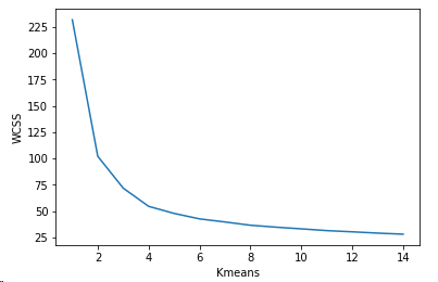
结论:数据集分成三个类别,一部分学生是决定继续读硕士,一部分放弃,还有一部分学生的比较犹豫,但是深造的可能性较大
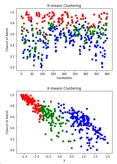
5.4.4 层次聚类
from scipy.cluster.hierarchy import linkage,dendrogram

merg = linkage(x,method='ward')

dendrogram(merg,leaf_rotation=90)

plt.xlabel('data points')

plt.ylabel('euclidean distance')

plt.show()

from sklearn.cluster import AgglomerativeClustering

hiyerartical_cluster = AgglomerativeClustering(n_clusters=3,affinity='euclidean',linkage='ward')

clusters_hiyerartical = hiyerartical_cluster.fit_predict(x)

df['label_hiyerartical'] = clusters_hiyerartical

plt.scatter(df[df.label_hiyerartical == 0 ]["Serial No."],df[df.label_hiyerartical == 0]['Chance of Admit'],color = "red")

plt.scatter(df[df.label_hiyerartical == 1 ]["Serial No."],df[df.label_hiyerartical == 1]['Chance of Admit'],color = "blue")

plt.scatter(df[df.label_hiyerartical == 2 ]["Serial No."],df[df.label_hiyerartical == 2]['Chance of Admit'],color = "green")

plt.title('Hierarchical Clustering')

plt.xlabel('Candidates')

plt.ylabel('Chance of Admit')

plt.show()

plt.scatter(data[df.label_hiyerartical == 0].x,data.y[df.label_hiyerartical==0],color='red')

plt.scatter(data[df.label_hiyerartical == 1].x,data.y[df.label_hiyerartical==1],color='blue')

plt.scatter(data[df.label_hiyerartical == 2].x,data.y[df.label_hiyerartical==2],color='green')

plt.title('Hierarchical Clustering')

plt.xlabel('X')

plt.ylabel('Chance of Admit')

plt.show()
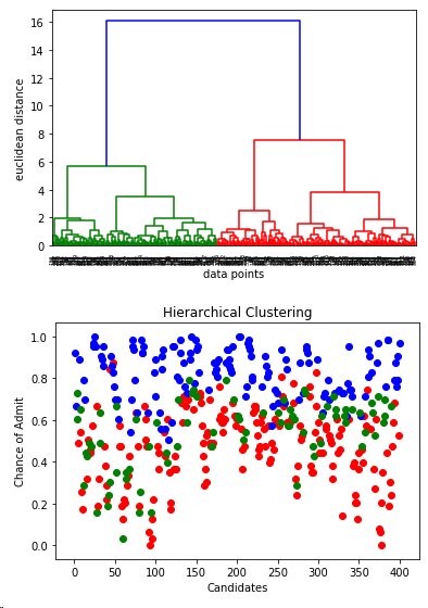

结论:从层次聚类的结果中,可以看出和K均值聚类的结果一致,只不过确定了聚类k的取值3
结论:通过本词入门数据集的训练,可以掌握
1.一些特征的展示的方法
2.如何调用sklearn 的API
3.如何取比较不同模型之间的好坏
代码+数据集:https://github.com/Mounment/python-data-analyze/tree/master/kaggle/score
如果有用的话,记得打一个星星,谢谢

Python-根据成绩分析是否继续深造的更多相关文章
- Python文章相关性分析---金庸武侠小说分析
百度到<金庸小说全集 14部>全(TXT)作者:金庸 下载下来,然后读取内容with open('names.txt') as f: data = [line.strip() for li ...
- [python]Python代码安全分析工具(Bandit)
简介: Bandit是一款Python源码分析框架,可用于Python代码的安全性分析.Bandit使用标准库中的ast模块,将Python源码解析成Python语法节点构成的树.Bandit允许用户 ...
- 用python探索和分析网络数据
Edited by Markdown Refered from: John Ladd, Jessica Otis, Christopher N. Warren, and Scott Weingart, ...
- python爬虫之分析Ajax请求抓取抓取今日头条街拍美图(七)
python爬虫之分析Ajax请求抓取抓取今日头条街拍美图 一.分析网站 1.进入浏览器,搜索今日头条,在搜索栏搜索街拍,然后选择图集这一栏. 2.按F12打开开发者工具,刷新网页,这时网页回弹到综合 ...
- Python文章相关性分析---金庸武侠小说分析-2018.1.16
最近常听同事提及相关性分析,正巧看到这个google的开源库,并把相关操作与调试结果记录下来. 输出结果: 比较有意思的巧合是黄蓉使出打狗棒,郭靖就用了降龙十八掌,再后测试了名词的解析. 小说集可以百 ...
- python 代码性能分析 库
问题描述 1.Python开发的程序在使用过程中很慢,想确定下是哪段代码比较慢: 2.Python开发的程序在使用过程中占用内存很大,想确定下是哪段代码引起的: 解决方案 使用profile分析分析c ...
- 使用flask做网页的excel成绩分析
使用到的技术:pyecharts flask 首先 pip install flask 和下载pip install pyecharts==0.5.5 项目结构: 代码: from flask imp ...
- 利用Python进行异常值分析实例代码
利用Python进行异常值分析实例代码 异常值是指样本中的个别值,也称为离群点,其数值明显偏离其余的观测值.常用检测方法3σ原则和箱型图.其中,3σ原则只适用服从正态分布的数据.在3σ原则下,异常值被 ...
- Python程序设计《集美大学各省成绩分析》
分析文件‘集美大学各省录取分数.xlsx’,完成以下功能: 1)集美大学2015-2018年间不同省份在本一批的平均分数,柱状图展示排名前10的省份, 2)分析福建省这3年各批次成绩情况,使用折线图展 ...
随机推荐
- 【转】NPOI使用手册
[转]NPOI使用手册 NPOI使用手册 目录 1.认识NPOI 2. 使用NPOI生成xls文件 2.1 创建基本内容 2.1.1创建Workbook和Sheet 2.1.2创建DocumentSu ...
- ArcSDE学习笔记------了解ArcSDE
刚来公司的时候一直在做地图服务,用的是ArcGIS,然后对地图的操作用的是普通的数据库操作.后来带我的一个同事让我学习一下ArcSDE.那么ArcSDE到底是什么呢?明明所有的操作我用普通数据库也实现 ...
- android 聊天室窗体
public class MainActivity extends Activity { ScrollView scrollView; Button button; LinearLayout layo ...
- Lesson 2 Building your first web page: Part 2
Tag Diagram You may have noticed that HTML tags come in pairs; HTML has both an opening tag (<tag ...
- BZOJ 3224 平衡树模板题
Treap: //By SiriusRen #include <cstdio> #include <algorithm> using namespace std; int n, ...
- 分享一个tom大叔的js 深入理解系列 (有助于提升)
http://www.cnblogs.com/TomXu/archive/2011/12/15/2288411.html#3620172
- Beautiful Number
http://acm.zju.edu.cn/onlinejudge/showProblem.do?problemCode=2829 Beautiful Number Time Limit: 2 Sec ...
- Windows 一键关闭UAC、防火墙、IE配置脚本
有时候,在环境需求下,需要关闭windows防火墙,UAC,以及IE选项配置. 对不懂电脑来说是比较麻烦的,老是得教他们,关键还记不住…… so,以下脚本就可以解决这个问题 注:脚本 需要右键 以管理 ...
- rm---删除目录huo文件
rm命令可以删除一个目录中的一个或多个文件或目录,也可以将某个目录及其下属的所有文件及其子目录均删除掉.对于链接文件,只是删除整个链接文件,而原有文件保持不变. 注意:使用rm命令要格外小心.因为一旦 ...
- 【Henu ACM Round#15 E】 A and B and Lecture Rooms
[链接] 我是链接,点我呀:) [题意] 在这里输入题意 [题解] 最近公共祖先. (树上倍增 一开始统计出每个子树的节点个数_size[i] 如果x和y相同. 那么直接输出n. 否则求出x和y的最近 ...