Convolutional Neural Network-week1编程题（TensorFlow实现手势数字识别）

1. TensorFlow model

import math
import numpy as np
import h5py
import matplotlib.pyplot as plt
import scipy
from PIL import Image
from scipy import ndimage
import tensorflow as tf
from tensorflow.python.framework import ops
from cnn_utils import *
%matplotlib inline
np.random.seed(1)

导入数据

# Loading the data (signs)
X_train_orig, Y_train_orig, X_test_orig, Y_test_orig, classes = load_dataset()

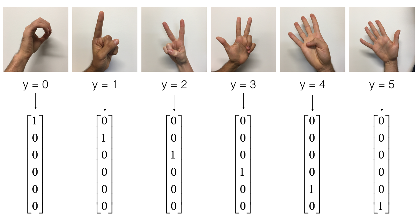
the SIGNS dataset is a collection of 6 signs representing numbers from 0 to 5.

展示数据

# Example of a picture
index = 6
plt.imshow(X_train_orig[index])
print ("y = " + str(np.squeeze(Y_train_orig[:, index])))

y = 2

数据的维度

X_train = X_train_orig/255.
X_test = X_test_orig/255.
Y_train = convert_to_one_hot(Y_train_orig, 6).T
Y_test = convert_to_one_hot(Y_test_orig, 6).T
print ("number of training examples = " + str(X_train.shape[0]))
print ("number of test examples = " + str(X_test.shape[0]))
print ("X_train shape: " + str(X_train.shape))
print ("Y_train shape: " + str(Y_train.shape))
print ("X_test shape: " + str(X_test.shape))
print ("Y_test shape: " + str(Y_test.shape))
conv_layers = {}

number of training examples = 1080

number of test examples = 120

X_train shape: (1080, 64, 64, 3)

Y_train shape: (1080, 6)

X_test shape: (120, 64, 64, 3)

Y_test shape: (120, 6)

1.1 Create placeholders

TensorFlow requires that you create placeholders for the input data that will be fed into the model when running the session.

Exercise: Implement the function below to create placeholders for the input image X and the output Y.

• You should not define the number of training examples for the moment.

• To do so, you could use "None" as the batch size, it will give you the flexibility to choose it later.

• Hence X should be of dimension [None, n_H0, n_W0, n_C0] and Y should be of dimension [None, n_y]. Hint.

# GRADED FUNCTION: create_placeholders
def create_placeholders(n_H0, n_W0, n_C0, n_y):
    """
    Creates the placeholders for the tensorflow session.
    Arguments:
    n_H0 -- scalar, height of an input image
    n_W0 -- scalar, width of an input image
    n_C0 -- scalar, number of channels of the input
    n_y -- scalar, number of classes
    Returns:
    X -- placeholder for the data input, of shape [None, n_H0, n_W0, n_C0] and dtype "float"
    Y -- placeholder for the input labels, of shape [None, n_y] and dtype "float"
    """
    ### START CODE HERE ### (≈2 lines)
    X = tf.placeholder(tf.float32, shape=[None, n_H0, n_W0, n_C0])
    Y = tf.placeholder(tf.float32, shape=[None, n_y])
    ### END CODE HERE ###
    return X, Y

测试：

X, Y = create_placeholders(64, 64, 3, 6)
print ("X = " + str(X))
print ("Y = " + str(Y))

输出：

X = Tensor("Placeholder:0", shape=(?, 64, 64, 3), dtype=float32)

Y = Tensor("Placeholder_1:0", shape=(?, 6), dtype=float32)

1.2 Initialize parameters

• You will initialize weights/filters \(W1\) and \(W2\) using tf.contrib.layers.xavier_initializer(seed = 0).

• You don't need to worry about bias variables as you will soon see that TensorFlow functions take care of the bias.

• Note also that you will only initialize the weights/filters for the conv2d functions. TensorFlow initializes the layers for the fully connected part automatically. We will talk more about that later in this assignment.

Exercise: Implement initialize_parameters(). The dimensions for each group of filters are provided below. Reminder - to initialize a parameter \(W\) of shape [1,2,3,4] in Tensorflow, use:

W = tf.get_variable("W", [1,2,3,4], initializer = ...)

More Info.

# GRADED FUNCTION: initialize_parameters
def initialize_parameters():
    """
    Initializes weight parameters to build a neural network with tensorflow. The shapes are:
                        W1 : [4, 4, 3, 8]
                        W2 : [2, 2, 8, 16]
    Returns:
    parameters -- a dictionary of tensors containing W1, W2
    """
    tf.set_random_seed(1)                              # so that your "random" numbers match ours
    ### START CODE HERE ### (approx. 2 lines of code)
    # (f, f, n_C_prev, n_C)
    W1 = tf.get_variable('W1',[4, 4, 3, 8], initializer = tf.contrib.layers.xavier_initializer(seed = 0))
    W2 = tf.get_variable('W2',[2, 2, 8, 16], initializer = tf.contrib.layers.xavier_initializer(seed = 0))
    ### END CODE HERE ###
    parameters = {"W1": W1,
                  "W2": W2}
    return parameters

测试

tf.reset_default_graph()
with tf.Session() as sess_test:
    parameters = initialize_parameters()
    init = tf.global_variables_initializer()
    sess_test.run(init)
    print("W1 = " + str(parameters["W1"].eval()[1,1,1]))
    print("W2 = " + str(parameters["W2"].eval()[1,1,1]))

1.2 Forward propagation

In TensorFlow, there are built-in functions that carry out the convolution steps for you.

• tf.nn.conv2d(X,W1, strides = [1,s,s,1], padding = 'SAME'): given an input \(X\) and a group of filters \(W1\), this function convolves \(W1\)'s filters on X. The third input ([1,f,f,1]) represents the strides for each dimension of the input (m, n_H_prev, n_W_prev, n_C_prev). You can read the full documentation here

• tf.nn.max_pool(A, ksize = [1,f,f,1], strides = [1,s,s,1], padding = 'SAME'): given an input A, this function uses a window of size (f, f) and strides of size (s, s) to carry out max pooling over each window. You can read the full documentation here

• tf.nn.relu(Z1): computes the elementwise ReLU of Z1 (which can be any shape). You can read the full documentation here.

• tf.contrib.layers.flatten(P): given an input P, this function flattens each example into a 1D vector it while maintaining the batch-size. It returns a flattened tensor with shape [batch_size, k]. You can read the full documentation here.

• tf.contrib.layers.fully_connected(F, num_outputs): given a the flattened input F, it returns the output computed using a fully connected layer. You can read the full documentation here.

In the last function above (tf.contrib.layers.fully_connected), the fully connected layer automatically initializes weights in the graph and keeps on training them as you train the model. Hence, you did not need to initialize those weights when initializing the parameters.

Exercise:

Implement the forward_propagation function below to build the following model: CONV2D -> RELU -> MAXPOOL -> CONV2D -> RELU -> MAXPOOL -> FLATTEN -> FULLYCONNECTED. You should use the functions above.

In detail, we will use the following parameters for all the steps:

• Conv2D: stride 1, padding is "SAME"

• ReLU

• Max pool: Use an 8 by 8 filter size and an 8 by 8 stride, padding is "SAME"

• Conv2D: stride 1, padding is "SAME"

• ReLU

• Max pool: Use a 4 by 4 filter size and a 4 by 4 stride, padding is "SAME"

• Flatten the previous output.

• FULLYCONNECTED (FC) layer: Apply a fully connected layer without an non-linear activation function. Do not call the softmax here. This will result in 6 neurons in the output layer, which then get passed later to a softmax. In TensorFlow, the softmax and cost function are lumped together into a single function, which you'll call in a different function when computing the cost.

# GRADED FUNCTION: forward_propagation
def forward_propagation(X, parameters):
    """
    Implements the forward propagation for the model:
    CONV2D -> RELU -> MAXPOOL -> CONV2D -> RELU -> MAXPOOL -> FLATTEN -> FULLYCONNECTED
    Arguments:
    X -- input dataset placeholder, of shape (input size, number of examples)
    parameters -- python dictionary containing your parameters "W1", "W2"
                  the shapes are given in initialize_parameters
    Returns:
    Z3 -- the output of the last LINEAR unit
    """
    # Retrieve the parameters from the dictionary "parameters"
    W1 = parameters['W1']
    W2 = parameters['W2']
    ### START CODE HERE ###
    # CONV2D: stride of 1, padding 'SAME'
    Z1 = tf.nn.conv2d(X, W1, strides = [1, 1, 1, 1], padding = 'SAME')
    # RELU
    A1 = tf.nn.relu(Z1)
    # MAXPOOL: window 8x8, sride 8, padding 'SAME'
    P1 = tf.nn.max_pool(A1, ksize = [1,8,8,1], strides = [1,8,8,1], padding = 'SAME')
    # CONV2D: filters W2, stride 1, padding 'SAME'
    Z2 = tf.nn.conv2d(P1,W2, strides = [1,1,1,1], padding = 'SAME')
    # RELU
    A2 = tf.nn.relu(Z2)
    # MAXPOOL: window 4x4, stride 4, padding 'SAME'
    P2 = tf.nn.max_pool(A2, ksize = [1,4,4,1], strides = [1,4,4,1], padding = 'SAME')
    # FLATTEN
    P2 = tf.contrib.layers.flatten(P2)
    # FULLY-CONNECTED without non-linear activation function (not not call softmax).
    # 6 neurons in output layer. Hint: one of the arguments should be "activation_fn=None"
    Z3 = tf.contrib.layers.fully_connected(P2, 6, activation_fn=None)
    ### END CODE HERE ###
    return Z3

测试：

tf.reset_default_graph()
with tf.Session() as sess:
    np.random.seed(1)
    X, Y = create_placeholders(64, 64, 3, 6)
    parameters = initialize_parameters()
    Z3 = forward_propagation(X, parameters)
    init = tf.global_variables_initializer()
    sess.run(init)
    a = sess.run(Z3, {X: np.random.randn(2,64,64,3), Y: np.random.randn(2,6)})
    print("Z3 = " + str(a))

1.3 Compute cost

Implement the compute cost function below. You might find these two functions helpful:

• tf.nn.softmax_cross_entropy_with_logits(logits = Z3, labels = Y):

  • computes the softmax entropy loss. This function both computes the softmax activation function as well as the resulting loss.

  • You can check the full documentation here.

• tf.reduce_mean: computes the mean of elements across dimensions of a tensor.

  • Use this to sum the losses over all the examples to get the overall cost. You can check the full documentation here.

** Exercise**: Compute the cost below using the function above.

# GRADED FUNCTION: compute_cost 
def compute_cost(Z3, Y):
    """
    Computes the cost
    Arguments:
    Z3 -- output of forward propagation (output of the last LINEAR unit), of shape (6, number of examples)
    Y -- "true" labels vector placeholder, same shape as Z3
    Returns:
    cost - Tensor of the cost function
    """
    ### START CODE HERE ### (1 line of code)
    cost = tf.nn.softmax_cross_entropy_with_logits(logits = Z3, labels = Y)
    cost = tf.reduce_mean(cost)
    ### END CODE HERE ###
    return cost

测试:

tf.reset_default_graph()
with tf.Session() as sess:
    np.random.seed(1)
    X, Y = create_placeholders(64, 64, 3, 6)
    parameters = initialize_parameters()
    Z3 = forward_propagation(X, parameters)
    cost = compute_cost(Z3, Y)
    init = tf.global_variables_initializer()
    sess.run(init)
    a = sess.run(cost, {X: np.random.randn(4,64,64,3), Y: np.random.randn(4,6)})
    print("cost = " + str(a))

cost = 2.91034

1.4 Model

Finally you will merge the helper functions you implemented above to build a model. You will train it on the SIGNS dataset.

You have implemented random_mini_batches() in the Optimization programming assignment of course 2. Remember that this function returns a list of mini-batches.

Exercise: Complete the function below.

The model below should:

• create placeholders
• initialize parameters
• forward propagate
• compute the cost
• create an optimizer

Finally you will create a session and run a for loop for num_epochs, get the mini-batches, and then for each mini-batch you will optimize the function. Hint for initializing the variables

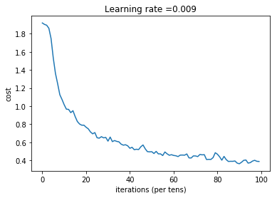
# GRADED FUNCTION: model
def model(X_train, Y_train, X_test, Y_test, learning_rate = 0.009,
          num_epochs = 100, minibatch_size = 64, print_cost = True):
    """
    Implements a three-layer ConvNet in Tensorflow:
    CONV2D -> RELU -> MAXPOOL -> CONV2D -> RELU -> MAXPOOL -> FLATTEN -> FULLYCONNECTED
    Arguments:
    X_train -- training set, of shape (None, 64, 64, 3)
    Y_train -- test set, of shape (None, n_y = 6)
    X_test -- training set, of shape (None, 64, 64, 3)
    Y_test -- test set, of shape (None, n_y = 6)
    learning_rate -- learning rate of the optimization
    num_epochs -- number of epochs of the optimization loop
    minibatch_size -- size of a minibatch
    print_cost -- True to print the cost every 100 epochs
    Returns:
    train_accuracy -- real number, accuracy on the train set (X_train)
    test_accuracy -- real number, testing accuracy on the test set (X_test)
    parameters -- parameters learnt by the model. They can then be used to predict.
    """
    ops.reset_default_graph()                         # to be able to rerun the model without overwriting tf variables
    tf.set_random_seed(1)                             # to keep results consistent (tensorflow seed)
    seed = 3                                          # to keep results consistent (numpy seed)
    (m, n_H0, n_W0, n_C0) = X_train.shape
    n_y = Y_train.shape[1]
    costs = []                                        # To keep track of the cost
    # Create Placeholders of the correct shape
    ### START CODE HERE ### (1 line)
    X, Y = create_placeholders(n_H0, n_W0, n_C0, n_y)
    ### END CODE HERE ###
    # Initialize parameters
    ### START CODE HERE ### (1 line)
    parameters = initialize_parameters()
    ### END CODE HERE ###
    # Forward propagation: Build the forward propagation in the tensorflow graph
    ### START CODE HERE ### (1 line)
    Z3 = forward_propagation(X, parameters)
    ### END CODE HERE ###
    # Cost function: Add cost function to tensorflow graph
    ### START CODE HERE ### (1 line)
    cost = compute_cost(Z3, Y)
    ### END CODE HERE ###
    # Backpropagation: Define the tensorflow optimizer. Use an AdamOptimizer that minimizes the cost.
    ### START CODE HERE ### (1 line)
    optimizer = tf.train.AdamOptimizer(learning_rate=learning_rate).minimize(cost)
    ### END CODE HERE ###
    # Initialize all the variables globally
    init = tf.global_variables_initializer()
    # Start the session to compute the tensorflow graph
    with tf.Session() as sess:
        # Run the initialization
        sess.run(init)
        # Do the training loop
        for epoch in range(num_epochs):
            minibatch_cost = 0.
            num_minibatches = int(m / minibatch_size) # number of minibatches of size minibatch_size in the train set
            seed = seed + 1
            minibatches = random_mini_batches(X_train, Y_train, minibatch_size, seed)
            for minibatch in minibatches:
                # Select a minibatch
                (minibatch_X, minibatch_Y) = minibatch
                # IMPORTANT: The line that runs the graph on a minibatch.
                # Run the session to execute the optimizer and the cost, the feedict should contain a minibatch for (X,Y).
                ### START CODE HERE ### (1 line)
                _ , temp_cost = sess.run([optimizer, cost], feed_dict={X: minibatch_X, Y: minibatch_Y})
                ### END CODE HERE ###
                minibatch_cost += temp_cost / num_minibatches
            # Print the cost every epoch
            if print_cost == True and epoch % 5 == 0:
                print ("Cost after epoch %i: %f" % (epoch, minibatch_cost))
            if print_cost == True and epoch % 1 == 0:
                costs.append(minibatch_cost)
        # plot the cost
        plt.plot(np.squeeze(costs))
        plt.ylabel('cost')
        plt.xlabel('iterations (per tens)')
        plt.title("Learning rate =" + str(learning_rate))
        plt.show()
        # Calculate the correct predictions
        predict_op = tf.argmax(Z3, 1)
        correct_prediction = tf.equal(predict_op, tf.argmax(Y, 1))
        # Calculate accuracy on the test set
        accuracy = tf.reduce_mean(tf.cast(correct_prediction, "float"))
        print(accuracy)
        train_accuracy = accuracy.eval({X: X_train, Y: Y_train})
        test_accuracy = accuracy.eval({X: X_test, Y: Y_test})
        print("Train Accuracy:", train_accuracy)
        print("Test Accuracy:", test_accuracy)
        return train_accuracy, test_accuracy, parameters

测试：

_, _, parameters = model(X_train, Y_train, X_test, Y_test)

Cost after epoch 0: 1.917920

Cost after epoch 5: 1.532475

Cost after epoch 10: 1.014804

Cost after epoch 15: 0.885137

Cost after epoch 20: 0.766963

Cost after epoch 25: 0.651208

Cost after epoch 30: 0.613356

Cost after epoch 35: 0.605931

Cost after epoch 40: 0.534713

Cost after epoch 45: 0.551402

Cost after epoch 50: 0.496976

Cost after epoch 55: 0.454438

Cost after epoch 60: 0.455496

Cost after epoch 65: 0.458359

Cost after epoch 70: 0.450040

Cost after epoch 75: 0.410687

Cost after epoch 80: 0.469005

Cost after epoch 85: 0.389253

Cost after epoch 90: 0.363808

Cost after epoch 95: 0.376132

Tensor("Mean_1:0", shape=(), dtype=float32)

Train Accuracy: 0.86851853

Test Accuracy: 0.73333335