CS190.1x-ML_lab3_linear_reg_student

这次作业主要是有关监督学习，数据集是来自UCI Machine Learning Repository的Million Song Dataset。我们的目的是训练一个线性回归的模型来预测一首歌的发行年份。相关ipynb文件见我github。

作业主要分成5个部分：读取和解析数据，创建模型和评价一个基础模型，训练和评估一个线性回归模型，用MLlib选择参数，增加交互项的特征。

Part 1 Read and parse the initial dataset

Load and check the data

读取数据，转换为RDD，看看数据前5个长啥样。

labVersion = 'cs190_week3_v_1_3'
# load testing library
from test_helper import Test
import os.path
baseDir = os.path.join('data')
inputPath = os.path.join('cs190', 'millionsong.txt')
fileName = os.path.join(baseDir, inputPath)

numPartitions = 2
rawData = sc.textFile(fileName, numPartitions)
# TODO: Replace <FILL IN> with appropriate code
numPoints = rawData.count()
print numPoints
samplePoints = rawData.take(5)
print samplePoints

samplePoints输出结果为

[u'2001.0,0.884123733793,0.610454259079,0.600498416968,0.474669212493,0.247232680947,0.357306088914,0.344136412234,0.339641227335,0.600858840135,0.425704689024,0.60491501652,0.419193351817', u'2001.0,0.854411946129,0.604124786151,0.593634078776,0.495885413963,0.266307830936,0.261472105188,0.506387076327,0.464453565511,0.665798573683,0.542968988766,0.58044428577,0.445219373624', u'2001.0,0.908982970575,0.632063159227,0.557428975183,0.498263761394,0.276396052336,0.312809861625,0.448530069406,0.448674249968,0.649791323916,0.489868662682,0.591908113534,0.4500023818', u'2001.0,0.842525219898,0.561826888508,0.508715259692,0.443531142139,0.296733836002,0.250213568176,0.488540873206,0.360508747659,0.575435243185,0.361005878554,0.678378718617,0.409036786173', u'2001.0,0.909303285534,0.653607720915,0.585580794716,0.473250503005,0.251417011835,0.326976795524,0.40432273022,0.371154511756,0.629401917965,0.482243251755,0.566901413923,0.463373691946']

Using LabeledPoint

在MLlib中，监督学习的记录存为LabeledPoint object。我们现在要写个函数，把RDD中的元素转换为LabeledPoint object。

from pyspark.mllib.regression import LabeledPoint
import numpy as np

# Here is a sample raw data point:
# '2001.0,0.884,0.610,0.600,0.474,0.247,0.357,0.344,0.33,0.600,0.425,0.60,0.419'
# In this raw data point, 2001.0 is the label, and the remaining values are features
# TODO: Replace <FILL IN> with appropriate code
def parsePoint(line):
    """Converts a comma separated unicode string into a `LabeledPoint`.

    Args:
        line (unicode): Comma separated unicode string where the first element is the label and the
            remaining elements are features.

    Returns:
        LabeledPoint: The line is converted into a `LabeledPoint`, which consists of a label and
            features.
    """
    return LabeledPoint(line.split(',')[0],line.split(',')[1:])

parsedSamplePoints = map(lambda x: parsePoint(x),samplePoints)
firstPointFeatures = parsedSamplePoints[0].features
firstPointLabel = parsedSamplePoints[0].label
print firstPointFeatures, firstPointLabel

d = len(firstPointFeatures)
print d

Visualization 1 Features

画了50个点的所有特征的灰度图

import matplotlib.pyplot as plt
import matplotlib.cm as cm

sampleMorePoints = rawData.take(50)
# You can uncomment the line below to see randomly selected features.  These will be randomly
# selected each time you run the cell.  Note that you should run this cell with the line commented
# out when answering the lab quiz questions.
# sampleMorePoints = rawData.takeSample(False, 50)

parsedSampleMorePoints = map(parsePoint, sampleMorePoints)
dataValues = map(lambda lp: lp.features.toArray(), parsedSampleMorePoints)

def preparePlot(xticks, yticks, figsize=(10.5, 6), hideLabels=False, gridColor='#999999',
                gridWidth=1.0):
    """Template for generating the plot layout."""
    plt.close()
    fig, ax = plt.subplots(figsize=figsize, facecolor='white', edgecolor='white')
    ax.axes.tick_params(labelcolor='#999999', labelsize='10')
    for axis, ticks in [(ax.get_xaxis(), xticks), (ax.get_yaxis(), yticks)]:
        axis.set_ticks_position('none')
        axis.set_ticks(ticks)
        axis.label.set_color('#999999')
        if hideLabels: axis.set_ticklabels([])
    plt.grid(color=gridColor, linewidth=gridWidth, linestyle='-')
    map(lambda position: ax.spines[position].set_visible(False), ['bottom', 'top', 'left', 'right'])
    return fig, ax

# generate layout and plot
fig, ax = preparePlot(np.arange(.5, 11, 1), np.arange(.5, 49, 1), figsize=(8,7), hideLabels=True,
                      gridColor='#eeeeee', gridWidth=1.1)
image = plt.imshow(dataValues,interpolation='nearest', aspect='auto', cmap=cm.Greys)
for x, y, s in zip(np.arange(-.125, 12, 1), np.repeat(-.75, 12), [str(x) for x in range(12)]):
    plt.text(x, y, s, color='#999999', size='10')
plt.text(4.7, -3, 'Feature', color='#999999', size='11'), ax.set_ylabel('Observation')
pass

Find the range

从标签里找到最大值和最小值。

# TODO: Replace <FILL IN> with appropriate code
parsedDataInit = rawData.map(lambda x: parsePoint(x))
onlyLabels = parsedDataInit.map(lambda x: x.label)
minYear = onlyLabels.takeOrdered(1)[0]
maxYear = onlyLabels.takeOrdered(1, key=lambda x: -x)[0]
print maxYear, minYear

Shift labels

转换特征，把最小的特征置为0.

# TODO: Replace <FILL IN> with appropriate code
parsedData = parsedDataInit.map(lambda x: LabeledPoint((x.label - minYear),x.features))

# Should be a LabeledPoint
print type(parsedData.take(1)[0])
# View the first point
print '\n{0}'.format(parsedData.take(1))

Training, validation, and test sets

这次用randomSplit()把数据随机分成三部分，记得缓存起来。

# TODO: Replace <FILL IN> with appropriate code
weights = [.8, .1, .1]
seed = 42
parsedTrainData, parsedValData, parsedTestData = parsedData.randomSplit(weights, seed)
parsedTrainData.cache()
parsedValData.cache()
parsedTestData.cache()
nTrain = parsedTrainData.count()
nVal = parsedValData.count()
nTest = parsedTestData.count()

print nTrain, nVal, nTest, nTrain + nVal + nTest
print parsedData.count()

Part 2 Create and evaluate a baseline model

Average label

我们首先想一个最简单的模型：Average label。主要思路是无论给什么入参，我们都给一样的判断：标签的平均值。

# TODO: Replace <FILL IN> with appropriate code
averageTrainYear = (parsedTrainData
                    .map(lambda x: x.label).sum() / float(nTrain))
print averageTrainYear

Root mean squared error

我们用RMSE来衡量一个模型的好坏。

# TODO: Replace <FILL IN> with appropriate code
def squaredError(label, prediction):
    """Calculates the the squared error for a single prediction.

    Args:
        label (float): The correct value for this observation.
        prediction (float): The predicted value for this observation.

    Returns:
        float: The difference between the `label` and `prediction` squared.
    """
    return (label - prediction)**2

def calcRMSE(labelsAndPreds):
    """Calculates the root mean squared error for an `RDD` of (label, prediction) tuples.

    Args:
        labelsAndPred (RDD of (float, float)): An `RDD` consisting of (label, prediction) tuples.

    Returns:
        float: The square root of the mean of the squared errors.
    """
    return np.sqrt((labelsAndPreds.map(lambda x:(x[0]-x[1])**2).sum())/labelsAndPreds.count())

labelsAndPreds = sc.parallelize([(3., 1.), (1., 2.), (2., 2.)])
# RMSE = sqrt[((3-1)^2 + (1-2)^2 + (2-2)^2) / 3] = 1.291
exampleRMSE = calcRMSE(labelsAndPreds)
print exampleRMSE

Training, validation and test RMSE

# TODO: Replace <FILL IN> with appropriate code
labelsAndPredsTrain = parsedTrainData.map(lambda lp:(lp.label,averageTrainYear))
rmseTrainBase = calcRMSE(labelsAndPredsTrain)

labelsAndPredsVal = parsedValData.map(lambda lp:(lp.label,averageTrainYear))
rmseValBase = calcRMSE(labelsAndPredsVal)

labelsAndPredsTest = parsedTestData.map(lambda lp:(lp.label,averageTrainYear))
rmseTestBase = calcRMSE(labelsAndPredsTest)

print 'Baseline Train RMSE = {0:.3f}'.format(rmseTrainBase)
print 'Baseline Validation RMSE = {0:.3f}'.format(rmseValBase)
print 'Baseline Test RMSE = {0:.3f}'.format(rmseTestBase)

Part 3 Train (via gradient descent) and evaluate a linear regression model

Gradient summand

from pyspark.mllib.linalg import DenseVector
# TODO: Replace <FILL IN> with appropriate code
def gradientSummand(weights, lp):
    """Calculates the gradient summand for a given weight and `LabeledPoint`.

    Note:
        `DenseVector` behaves similarly to a `numpy.ndarray` and they can be used interchangably
        within this function.  For example, they both implement the `dot` method.

    Args:
        weights (DenseVector): An array of model weights (betas).
        lp (LabeledPoint): The `LabeledPoint` for a single observation.

    Returns:
        DenseVector: An array of values the same length as `weights`.  The gradient summand.
    """
    x = lp.features
    y = lp.label
    summand = (np.dot(weights,x) -y ) * x
    return summand

exampleW = DenseVector([1, 1, 1])
exampleLP = LabeledPoint(2.0, [3, 1, 4])
# gradientSummand = (dot([1 1 1], [3 1 4]) - 2) * [3 1 4] = (8 - 2) * [3 1 4] = [18 6 24]
summandOne = gradientSummand(exampleW, exampleLP)
print summandOne

exampleW = DenseVector([.24, 1.2, -1.4])
exampleLP = LabeledPoint(3.0, [-1.4, 4.2, 2.1])
summandTwo = gradientSummand(exampleW, exampleLP)
print summandTwo

Use weights to make predictions

# TODO: Replace <FILL IN> with appropriate code
def getLabeledPrediction(weights, observation):
    """Calculates predictions and returns a (label, prediction) tuple.

    Note:
        The labels should remain unchanged as we'll use this information to calculate prediction
        error later.

    Args:
        weights (np.ndarray): An array with one weight for each features in `trainData`.
        observation (LabeledPoint): A `LabeledPoint` that contain the correct label and the
            features for the data point.

    Returns:
        tuple: A (label, prediction) tuple.
    """
    return (observation.label,np.dot(weights,observation.features))

weights = np.array([1.0, 1.5])
predictionExample = sc.parallelize([LabeledPoint(2, np.array([1.0, .5])),
                                    LabeledPoint(1.5, np.array([.5, .5]))])
labelsAndPredsExample = predictionExample.map(lambda lp: getLabeledPrediction(weights, lp))
print labelsAndPredsExample.collect()

Gradient descent

这次作业最难地方就是实现梯度下降。

# TODO: Replace <FILL IN> with appropriate code
def linregGradientDescent(trainData, numIters):
    """Calculates the weights and error for a linear regression model trained with gradient descent.

    Note:
        `DenseVector` behaves similarly to a `numpy.ndarray` and they can be used interchangably
        within this function.  For example, they both implement the `dot` method.

    Args:
        trainData (RDD of LabeledPoint): The labeled data for use in training the model.
        numIters (int): The number of iterations of gradient descent to perform.

    Returns:
        (np.ndarray, np.ndarray): A tuple of (weights, training errors).  Weights will be the
            final weights (one weight per feature) for the model, and training errors will contain
            an error (RMSE) for each iteration of the algorithm.
    """
    # The length of the training data
    n = trainData.count()
    # The number of features in the training data
    d = len(trainData.take(1)[0].features)
    w = np.zeros(d)
    alpha = 1.0
    # We will compute and store the training error after each iteration
    errorTrain = np.zeros(numIters)
    for i in range(numIters):
        # Use getLabeledPrediction from (3b) with trainData to obtain an RDD of (label, prediction)
        # tuples.  Note that the weights all equal 0 for the first iteration, so the predictions will
        # have large errors to start.
        labelsAndPredsTrain = trainData.map(lambda lp: getLabeledPrediction(w, lp))
        errorTrain[i] = calcRMSE(labelsAndPredsTrain)

        # Calculate the `gradient`.  Make use of the `gradientSummand` function you wrote in (3a).
        # Note that `gradient` sould be a `DenseVector` of length `d`.
        gradient = trainData.map(lambda lp:gradientSummand(DenseVector(w),lp)).sum()

        # Update the weights
        alpha_i = alpha / (n * np.sqrt(i+1))
        w -= alpha_i * gradient
    return w, errorTrain

# create a toy dataset with n = 10, d = 3, and then run 5 iterations of gradient descent
# note: the resulting model will not be useful; the goal here is to verify that
# linregGradientDescent is working properly
exampleN = 10
exampleD = 3
exampleData = (sc
               .parallelize(parsedTrainData.take(exampleN))
               .map(lambda lp: LabeledPoint(lp.label, lp.features[0:exampleD])))
print exampleData.take(2)
exampleNumIters = 5
exampleWeights, exampleErrorTrain = linregGradientDescent(exampleData, exampleNumIters)
print exampleWeights

Train the model

# TODO: Replace <FILL IN> with appropriate code
numIters = 50
weightsLR0, errorTrainLR0 = linregGradientDescent(parsedTrainData,numIters)

labelsAndPreds = parsedValData.map(lambda lp:getLabeledPrediction(weightsLR0,lp))
rmseValLR0 = calcRMSE(labelsAndPreds)

print 'Validation RMSE:\n\tBaseline = {0:.3f}\n\tLR0 = {1:.3f}'.format(rmseValBase,
                                                                       rmseValLR0)

Part 4 Train using MLlib and perform grid search

事实上，MLlib里面提供了LinearRegressionWithSGD来实现上面的算法，而且功能更强大，比如选择随机梯度算法，以及加L1和L2正则化。

from pyspark.mllib.regression import LinearRegressionWithSGD
# Values to use when training the linear regression model
numIters = 500  # iterations
alpha = 1.0  # step
miniBatchFrac = 1.0  # miniBatchFraction
reg = 1e-1  # regParam
regType = 'l2'  # regType
useIntercept = True  # intercept
# TODO: Replace <FILL IN> with appropriate code
firstModel = LinearRegressionWithSGD.train(parsedTrainData, iterations=numIters, step=alpha,
                                           miniBatchFraction=miniBatchFrac, initialWeights=None, regParam=reg, regType=regType,
                                          intercept=useIntercept)

# weightsLR1 stores the model weights; interceptLR1 stores the model intercept
weightsLR1 = firstModel.weights
interceptLR1 = firstModel.intercept
print weightsLR1, interceptLR1

Predict

这里我们用MLlib提供的LinearRegressionModel.predict()方法来预测。

# TODO: Replace <FILL IN> with appropriate code
samplePoint = parsedTrainData.take(1)[0]
samplePrediction = firstModel.predict(samplePoint.features)
print samplePrediction

Evaluate RMSE

# TODO: Replace <FILL IN> with appropriate code
labelsAndPreds = parsedValData.map(lambda lp:(lp.label,firstModel.predict(lp.features)))
rmseValLR1 = calcRMSE(labelsAndPreds)

print ('Validation RMSE:\n\tBaseline = {0:.3f}\n\tLR0 = {1:.3f}' +
       '\n\tLR1 = {2:.3f}').format(rmseValBase, rmseValLR0, rmseValLR1)

Grid search

我们要改进上面的结果，比如正则化的参数试试1e-10, 1e-5, and 1。

# TODO: Replace <FILL IN> with appropriate code
bestRMSE = rmseValLR1
bestRegParam = reg
bestModel = firstModel

numIters = 500
alpha = 1.0
miniBatchFrac = 1.0
for reg in (1e-10,1e-5,1):
    model = LinearRegressionWithSGD.train(parsedTrainData, numIters, alpha,
                                          miniBatchFrac, regParam=reg,
                                          regType='l2', intercept=True)
    labelsAndPreds = parsedValData.map(lambda lp: (lp.label, model.predict(lp.features)))
    rmseValGrid = calcRMSE(labelsAndPreds)
    print rmseValGrid

    if rmseValGrid < bestRMSE:
        bestRMSE = rmseValGrid
        bestRegParam = reg
        bestModel = model
rmseValLRGrid = bestRMSE

print ('Validation RMSE:\n\tBaseline = {0:.3f}\n\tLR0 = {1:.3f}\n\tLR1 = {2:.3f}\n' +
       '\tLRGrid = {3:.3f}').format(rmseValBase, rmseValLR0, rmseValLR1, rmseValLRGrid)

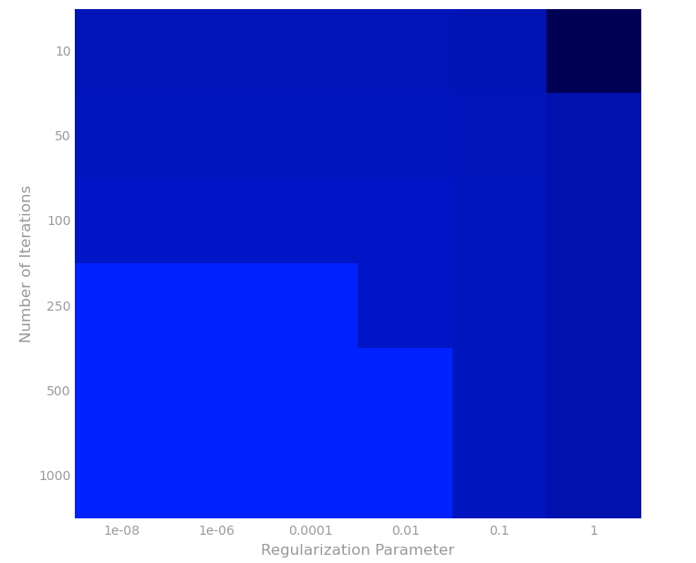
Vary alpha and the number of iterations

这次我们试试找alpha和迭代次数的其他值的情况下的RMSE。

# TODO: Replace <FILL IN> with appropriate code
reg = bestRegParam
modelRMSEs = []

for alpha in (1e-5,10):
    for numIters in (500,5):
        model = LinearRegressionWithSGD.train(parsedTrainData, numIters, alpha,
                                              miniBatchFrac, regParam=reg,
                                              regType='l2', intercept=True)
        labelsAndPreds = parsedValData.map(lambda lp: (lp.label, model.predict(lp.features)))
        rmseVal = calcRMSE(labelsAndPreds)
        print 'alpha = {0:.0e}, numIters = {1}, RMSE = {2:.3f}'.format(alpha, numIters, rmseVal)
        modelRMSEs.append(rmseVal)

通过上面结果，可以画出如下图。

Part 5 Add interactions between features

Add 2-way interactions

这里我们加一些交互项进去，这是线性回归很常见的做法，可以增加模型的复杂度。我们可以用itertools.product来产生2-way interaction。

# TODO: Replace <FILL IN> with appropriate code
import itertools

def twoWayInteractions(lp):
    """Creates a new `LabeledPoint` that includes two-way interactions.

    Note:
        For features [x, y] the two-way interactions would be [x^2, x*y, y*x, y^2] and these
        would be appended to the original [x, y] feature list.

    Args:
        lp (LabeledPoint): The label and features for this observation.

    Returns:
        LabeledPoint: The new `LabeledPoint` should have the same label as `lp`.  Its features
            should include the features from `lp` followed by the two-way interaction features.
    """
    origLabel = lp.label
    origFeatures = lp.features
    twoWayFeatures = map(lambda (x,y):x*y ,itertools.product(origFeatures,repeat=2))
    return LabeledPoint(origLabel,np.hstack((origFeatures,twoWayFeatures)))

print twoWayInteractions(LabeledPoint(0.0, [2, 3]))

# Transform the existing train, validation, and test sets to include two-way interactions.
trainDataInteract = parsedTrainData.map(lambda lp: twoWayInteractions(lp)).cache()
valDataInteract = parsedValData.map(lambda lp: twoWayInteractions(lp)).cache()
testDataInteract = parsedTestData.map(lambda lp: twoWayInteractions(lp)).cache()

Build interaction model

我们增加了新的特征后，重新训练模型。

# TODO: Replace <FILL IN> with appropriate code
numIters = 500
alpha = 1.0
miniBatchFrac = 1.0
reg = 1e-10

modelInteract = LinearRegressionWithSGD.train(trainDataInteract, numIters, alpha,
                                              miniBatchFrac, regParam=reg,
                                              regType='l2', intercept=True)
labelsAndPredsInteract = valDataInteract.map(lambda lp: (lp.label, modelInteract.predict(lp.features)))
rmseValInteract = calcRMSE(labelsAndPredsInteract)

print ('Validation RMSE:\n\tBaseline = {0:.3f}\n\tLR0 = {1:.3f}\n\tLR1 = {2:.3f}\n\tLRGrid = ' +
       '{3:.3f}\n\tLRInteract = {4:.3f}').format(rmseValBase, rmseValLR0, rmseValLR1,
                                                 rmseValLRGrid, rmseValInteract)

Evaluate interaction model on test data

# TODO: Replace <FILL IN> with appropriate code
labelsAndPredsTest = testDataInteract.map(lambda lp: (lp.label, modelInteract.predict(lp.features)))
rmseTestInteract = calcRMSE(labelsAndPredsTest)

print ('Test RMSE:\n\tBaseline = {0:.3f}\n\tLRInteract = {1:.3f}'
       .format(rmseTestBase, rmseTestInteract))

我们发现无论是训练的RMSE还是测试集上的RMSE，均比之前的模型要好。