tensorflow实现LeNet-5模型

网络结构如下：

INPUT: [28x28x1]           weights: 0
CONV5-32: [28x28x32]       weights: (5*5*1+1)*32
POOL2: [14x14x32]          weights: 0
CONV5-64: [14x14x64]       weights: (5*5*32+1)*64
POOL2: [7x7x64]          weights: 0
FC: [1x1x512]              weights: (7*7*64+1)*512
FC: [1x1x10]              weights: (1*1*512+1)*1

工程目录：

-mnist_lenet5
    -dataset  //存放数据集的文件夹，可以http://yann.lecun.com/exdb/mnist/下载
    -model   //存放模型的文件夹
    -mnist_eval.py  //定义了测试过程
    -mnist_inference.py  //定义了前向传播的过程以及神经网络中的参数
    -mnist_train.py     //定义了神经网络的训练过程

mnist_eval.py

# -*- coding: utf-8 -*-
import time
import numpy as np
import tensorflow as tf
from tensorflow.examples.tutorials.mnist import input_data
 
# 加载mnist_inference.py 和 mnist_train.py中定义的常量和函数
import mnist_inference
import mnist_train
 
# 每10秒加载一次最新的模型， 并在测试数据上测试最新模型的正确率
EVAL_INTERVAL_SECS = 1
 
def evaluate(mnist):
    with tf.Graph().as_default() as g:
        # 定义输入输出的格式
        x = tf.placeholder(tf.float32, [
            mnist.validation.num_examples,           # 第一维表示样例的个数
            mnist_inference.IMAGE_SIZE,             # 第二维和第三维表示图片的尺寸
            mnist_inference.IMAGE_SIZE,
            mnist_inference.NUM_CHANNELS],          # 第四维表示图片的深度，对于RBG格式的图片，深度为5
                       name='x-input')
        y_ = tf.placeholder(tf.float32, [None, mnist_inference.OUTPUT_NODE], name='y-input')
 
        validate_feed = {x: np.reshape(mnist.validation.images, (mnist.validation.num_examples, mnist_inference.IMAGE_SIZE, mnist_inference.IMAGE_SIZE, mnist_inference.NUM_CHANNELS)),
                         y_: mnist.validation.labels}
        # 直接通过调用封装好的函数来计算前向传播的结果。
        # 因为测试时不关注正则损失的值，所以这里用于计算正则化损失的函数被设置为None。
        y = mnist_inference.inference(x, False, None)
 
        # 使用前向传播的结果计算正确率。
        # 如果需要对未知的样例进行分类，那么使用tf.argmax(y, 1)就可以得到输入样例的预测类别了。
        correct_prediction = tf.equal(tf.argmax(y, 1), tf.argmax(y_, 1))
        accuracy = tf.reduce_mean(tf.cast(correct_prediction, tf.float32))
 
        # 通过变量重命名的方式来加载模型，这样在前向传播的过程中就不需要调用求滑动平均的函数来获取平局值了。
        # 这样就可以完全共用mnist_inference.py中定义的前向传播过程
        variable_averages = tf.train.ExponentialMovingAverage(mnist_train.MOVING_AVERAGE_DECAY)
        variable_to_restore = variable_averages.variables_to_restore()
        saver = tf.train.Saver(variable_to_restore)
 
        #每隔EVAL_INTERVAL_SECS秒调用一次计算正确率的过程以检测训练过程中正确率的变化
        while True:
            with tf.Session() as sess:
                # tf.train.get_checkpoint_state函数会通过checkpoint文件自动找到目录中最新模型的文件名
                ckpt = tf.train.get_checkpoint_state(mnist_train.MODEL_SAVE_PATH)
                if ckpt and ckpt.model_checkpoint_path:
                    # 加载模型
                    saver.restore(sess, ckpt.model_checkpoint_path)
                    # 通过文件名得到模型保存时迭代的轮数
                    global_step = ckpt.model_checkpoint_path.split('/')[-1].split('-')[-1]
                    accuracy_score = sess.run(accuracy, feed_dict = validate_feed)
                    print("After %s training step(s), validation accuracy = %f" % (global_step, accuracy_score))
                else:
                    print("No checkpoint file found")
                    return
            time.sleep(EVAL_INTERVAL_SECS)
 
if __name__ == '__main__':
    mnist = input_data.read_data_sets("E:/MNIST_data", one_hot=True)
    evaluate(mnist)

mnist_inference.py

# -*- coding: utf-8 -*-
 
import tensorflow as tf
 
# 定义神经网络相关的参数
INPUT_NODE = 784
OUTPUT_NODE = 10
LAYER1_NODE = 500
 
IMAGE_SIZE = 28
NUM_CHANNELS = 1
NUM_LABELS = 10
 
# 第一层卷积层的尺寸和深度
CONV1_DEEP = 32
CONV1_SIZE = 5
# 第二层卷积层的尺寸和深度
CONV2_DEEP = 64
CONV2_SIZE = 5
# 全连接层的节点个数
FC_SIZE = 512
 
# 定义神经网络的前向传播过程。
# 这里添加了一个新的参数train，用于区别训练过程和测试过程。
# 在这个程序中将用到dropout方法，dropout可以进一步提升模型可靠性并防止过拟合，dropout过程只在训练时使用。
def inference(input_tensor, train, regularizer):
    # 声明第一层神经网络的变量并完成前向传播过程。这个过程和6.3.1小节中介绍的一致。
    # 通过使用不同的命名空间来隔离不同层的变量，这可以让每一层中的变量命名只需要考虑在当前层的作用，而不需要担心重名的问题。
    # 和标准LeNet-5模型不大一样，这里定义卷积层的输入为28*28*1的原始MNIST图片像素。
    # 因为卷积层中使用了全0填充，所以输出为28*28*32的矩阵。
    with tf.variable_scope('layer1-conv1'):
        # 这里使用tf.get_variable或tf.Variable没有本质区别，因为在训练或是测试中没有在同一个程序中多次调用这个函数。
        # 如果在同一个程序中多次调用，在第一次调用之后需要将reuse参数置为True。
        conv1_weights = tf.get_variable(
            "weight", [CONV1_SIZE, CONV1_SIZE, NUM_CHANNELS, CONV1_DEEP],
            initializer = tf.truncated_normal_initializer(stddev=0.1)
        )
        conv1_biases = tf.get_variable("bias", [CONV1_DEEP], initializer=tf.constant_initializer(0.0))
        # 使用边长为5，深度为32的过滤器，过滤器移动的步长为1，且使用全0填充
        conv1 = tf.nn.conv2d(input_tensor, conv1_weights, strides=[1, 1, 1, 1], padding='SAME')
        relu1 = tf.nn.relu(tf.nn.bias_add(conv1, conv1_biases))
 
    # 实现第二层池化层的前向传播过程。
    # 这里选用最大池化层，池化层过滤器的边长为2，使用全0填充且移动的步长为2。
    # 这一层的输入是上一层的输出，也就是28*28*32的矩阵。输出为14*14*32的矩阵。
    with tf.name_scope('layer2-pool'):
        pool1 = tf.nn.max_pool(relu1, ksize=[1, 2, 2, 1], strides=[1, 2, 2, 1], padding='SAME')
 
    # 声明第三层卷积层的变量并实现前向传播过程。
    # 这一层的输入为14*14*32的矩阵，输出为14*14*64的矩阵。
    with tf.variable_scope('layer3-conv2'):
        conv2_weights = tf.get_variable(
            "weight", [CONV2_SIZE, CONV2_SIZE, CONV1_DEEP, CONV2_DEEP],
            initializer = tf.truncated_normal_initializer(stddev=0.1)
        )
        conv2_biases = tf.get_variable("bias", [CONV2_DEEP], initializer=tf.constant_initializer(0.0))
        # 使用边长为5，深度为64的过滤器，过滤器移动的步长为1，且使用全0填充
        conv2 = tf.nn.conv2d(pool1, conv2_weights, strides=[1, 1, 1, 1], padding='SAME')
        relu2 = tf.nn.relu(tf.nn.bias_add(conv2, conv2_biases))
 
    # 实现第四层池化层的前向传播过程。
    # 这一层和第二层的结构是一样的。这一层的输入为14*14*64的矩阵，输出为7*7*64的矩阵。
    with tf.name_scope('layer4-poo2'):
        pool2 = tf.nn.max_pool(relu2, ksize=[1, 2, 2, 1], strides=[1, 2, 2, 1], padding='SAME')
 
    # 将第四层池化层的输出转化为第五层全连接层的输入格式。
    # 第四层的输出为7*7*64的矩阵，然而第五层全连接层需要的输入格式为向量，所以在这里需要将这个7*7*64的矩阵拉直成一个向量。
    # pool2.get_shape函数可以得到第四层输出矩阵的维度而不需要手工计算。
    # 注意因为每一层神经网络的输入输出都为一个batch的矩阵，所以这里得到的维度也包含了一个batch中数据的个数。
    pool_shape = pool2.get_shape().as_list()
    # 计算将矩阵拉直成向量之后的长度，这个长度就是矩阵长度及深度的乘积。
    # 注意这里pool_shape[0]为一个batch中样本的个数。
    nodes = pool_shape[1] * pool_shape[2] * pool_shape[3]
    # 通过tf.reshape函数将第四层的输出变成一个batch的向量。
    reshaped = tf.reshape(pool2, [pool_shape[0], nodes])
 
    # 声明第五层全连接层的变量并实现前向传播过程。
    # 这一层的输入是拉直之后的一组向量，向量长度为7*7*64=3136，输出是一组长度为512的向量。
    # 这一层和之前在第5章中介绍的基本一致，唯一的区别是引入了dropout的概念。
    # dropout在训练时会随机将部分节点的输出改为0。
    # dropout可以避免过拟合问题，从而使得模型在测试数据上的效果更好。
    # dropout一般只在全连接层而不是卷积层或者池化层使用。
    with tf.variable_scope('layer5-fc1'):
        fc1_weights = tf.get_variable("weight", [nodes, FC_SIZE],
                                      initializer = tf.truncated_normal_initializer(stddev = 0.1))
        # 只有全连接层的权重需要加入正则化
        if regularizer != None:
            tf.add_to_collection('losses', regularizer(fc1_weights))
        fc1_biases = tf.get_variable('bias', [FC_SIZE], initializer = tf.constant_initializer(0.1))
        fc1 = tf.nn.relu(tf.matmul(reshaped, fc1_weights)+fc1_biases)
        if train:
            fc1 = tf.nn.dropout(fc1, 0.5)
 
    # 声明第六层全连接层的变量并实现前向传播过程。
    # 这一层的输入是一组长度为512的向量，输出是一组长度为10的向量。
    # 这一层的输出通过Softmax之后就得到了最后的分类结果。
    with tf.variable_scope('layer6-fc2'):
        fc2_weights = tf.get_variable("weight", [FC_SIZE, NUM_LABELS],
                                      initializer = tf.truncated_normal_initializer(stddev = 0.1))
        if regularizer != None:
            tf.add_to_collection('losses', regularizer(fc2_weights))
        fc2_biases = tf.get_variable('bias', [NUM_LABELS], initializer = tf.constant_initializer(0.1))
        logit = tf.matmul(fc1, fc2_weights) + fc2_biases
 
    # 返回第六层的输出
    return logit

mnist_train.py

# -*- coding: utf-8 -*-
import os
import numpy as np
 
import tensorflow as tf
from tensorflow.examples.tutorials.mnist import input_data
 
# 加载mnist_inference.py中定义的常量和前向传播的函数
import mnist_inference
 
# 配置神经网络的参数
BATCH_SIZE = 100
LEARNING_RATE_BASE = 0.01
LEARNING_RATE_DECAY = 0.99
REGULARAZTION_RATE = 0.0001
TRAINING_STEPS = 300
MOVING_AVERAGE_DECAY = 0.99
# 模型保存的路径和文件名
MODEL_SAVE_PATH = "model/"
MODEL_NAME = "model.ckpt"
 
def train(mnist):
    # 定义输入输出placeholder
    # 调整输入数据placeholder的格式，输入为一个四维矩阵
    x = tf.placeholder(tf.float32, [
        BATCH_SIZE,  # 第一维表示一个batch中样例的个数
        mnist_inference.IMAGE_SIZE,  # 第二维和第三维表示图片的尺寸
        mnist_inference.IMAGE_SIZE,
        mnist_inference.NUM_CHANNELS],  # 第四维表示图片的深度，对于RBG格式的图片，深度为5
                       name='x-input')
    y_ = tf.placeholder(tf.float32, [None, mnist_inference.OUTPUT_NODE], name='y-input')
 
    regularizer = tf.contrib.layers.l2_regularizer(REGULARAZTION_RATE)
    # 直接使用mnist_inference.py中定义的前向传播过程
    y = mnist_inference.inference(x, True, regularizer)
    global_step = tf.Variable(0, trainable=False)
 
    # 定义损失函数、学习率、滑动平均操作以及训练过程
    variable_averages = tf.train.ExponentialMovingAverage(MOVING_AVERAGE_DECAY, global_step)
    variable_averages_op = variable_averages.apply(tf.trainable_variables())
    cross_entropy = tf.nn.sparse_softmax_cross_entropy_with_logits(logits=y, labels=tf.argmax(y_, 1))
    cross_entropy_mean = tf.reduce_mean(cross_entropy)
    loss = cross_entropy_mean + tf.add_n(tf.get_collection('losses'))
    learning_rate = tf.train.exponential_decay(LEARNING_RATE_BASE, global_step, mnist.train.num_examples / BATCH_SIZE, LEARNING_RATE_DECAY)
    train_step = tf.train.GradientDescentOptimizer(learning_rate).minimize(loss, global_step=global_step)
    with tf.control_dependencies([train_step, variable_averages_op]):
        train_op = tf.no_op(name='train')
 
    # 初始化Tensorflow持久化类
    saver = tf.train.Saver()
    with tf.Session() as sess:
        tf.global_variables_initializer().run()
        # 验证和测试的过程将会有一个独立的程序来完成
        for i in range(TRAINING_STEPS):
            xs, ys = mnist.train.next_batch(BATCH_SIZE)
            # 类似地将输入的训练数据格式调整为一个四维矩阵，并将这个调整后的数据传入sess.run过程
            reshaped_xs = np.reshape(xs, (BATCH_SIZE, mnist_inference.IMAGE_SIZE, mnist_inference.IMAGE_SIZE, mnist_inference.NUM_CHANNELS))
            _, loss_value, step = sess.run([train_op, loss, global_step], feed_dict={x: reshaped_xs, y_: ys})
            # 每1000轮保存一次模型。
            if i % 1 == 0:
                # 输出当前的训练情况。这里只输出了模型在当前训练batch上的损失函数大小。通过损失函数的大小可以大概了解训练的情况。
                # 在验证数据集上的正确率信息会有一个单独的程序来生成。
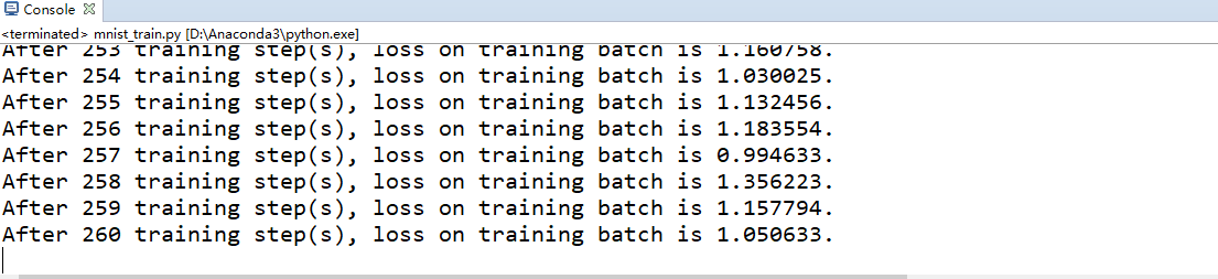
                print("After %d training step(s), loss on training batch is %f." % (step, loss_value))
                # 保存当前的模型。注意这里隔出了global_step参数，这样可以让每个被保存模型的文件名末尾加上训练的轮数，比如“model.ckpt-1000”表示训练1000轮后得到的模型
                saver.save(sess, os.path.join(MODEL_SAVE_PATH, MODEL_NAME), global_step=global_step)
 
if __name__ == '__main__':
    mnist = input_data.read_data_sets("E:/MNIST_data", one_hot=True)
    train(mnist)

转自：http://blog.csdn.net/nnnnnnnnnnnny/article/details/70216265