Opencv之LBP特征(算法)
LBP(Local Binary Pattern),即局部二进制模式,对一个像素点以半径r画一个圈,在圈上取K个点(一般为8),这K个点的值(像素值大于中心点为1,否则为0)组成K位二进制数。此即局部二进制模式,实际中使用的是LBP特征谱的直方统计图。在旧版的Opencv里,使用CvHaarClassifierCascade函数,只支持Harr特征。新版使用CascadeClassifier类,还可以支持LBP特征。Opencv的人脸识别使用的是Extended LBP(即circle_LBP),其LBP特征值的模式为256(0-255)种。
优点:
1,旋转不变性(局部二进制循环左移或右移其表示不变)
2,一定程度上消除了光照变化的问题
3,纹理特征维度低,计算速度快
缺点:
1,当光照变化不均匀时,各像素间的大小关系被破坏,对应的LBP算子也就发生了变化
2,通过引入旋转不变的定义,使LBP算子更具鲁棒性。但这也使得LBP算子丢失了方向信息(如使局部二进制左移或右移,结果是一样的,但是图像不一样)
以下介绍若干中LBP:
1,原始LBP。基于方框选取中心点周围8个像素,构成8位二进制
# 以下不再重复这个部分

import cv2

import numpy as np

image_path=your_img_path
# 原始LBP算法:选取中心点周围的8个像素点,大于中心点为1,小于为0,将这些1或0顺时针串成8位二进制,即最终表示

def origin_LBP(img):

    dst = np.zeros(img.shape,dtype=img.dtype)

    h,w=img.shape

    start_index=1

    for i in range(start_index,h-1):

        for j in range(start_index,w-1):

            center = img[i][j]

            code = 0

#             顺时针,左上角开始的8个像素点与中心点比较,大于等于的为1,小于的为0,最后组成8位2进制

            code |= (img[i-1][j-1] >= center) << (np.uint8)(7)

            code |= (img[i-1][j  ] >= center) << (np.uint8)(6)

            code |= (img[i-1][j+1] >= center) << (np.uint8)(5)

            code |= (img[i  ][j+1] >= center) << (np.uint8)(4)

            code |= (img[i+1][j+1] >= center) << (np.uint8)(3)

            code |= (img[i+1][j  ] >= center) << (np.uint8)(2)

            code |= (img[i+1][j-1] >= center) << (np.uint8)(1)

            code |= (img[i  ][j-1] >= center) << (np.uint8)(0)

            dst[i-start_index][j-start_index]= code

    return dst

# 读入灰度图

gray = cv2.imread(image_path, cv2.IMREAD_GRAYSCALE)

# LBP处理

org_lbp = origin_LBP(gray)
cv2.imshow('img', gray)

cv2.imshow('org_lbp', org_lbp)

# 若针对视频取图片,delay=k时表示下一帧在kms后选取

cv2.waitKey(0)
2,Extended LBP
# 使用圆形选取框替代矩形框选:给定半径为r(半径越小,纹理越细),在此圆上选择K个点(选取点越多,亮度越高),同样,逆/顺时针组成K为二进制

# 称为extend LBP

def circular_LBP(img, radius=3, neighbors=8):

    h,w=img.shape

    dst = np.zeros((h-2*radius, w-2*radius),dtype=img.dtype)

    for i in range(radius,h-radius):

        for j in range(radius,w-radius):

            # 获得中心像素点的灰度值

            center = img[i,j]

            for k in range(neighbors):

                # 计算采样点对于中心点坐标的偏移量rx,ry

                rx = radius * np.cos(2.0 * np.pi * k / neighbors)

                ry = -(radius * np.sin(2.0 * np.pi * k / neighbors))

                # 为双线性插值做准备

                # 对采样点偏移量分别进行上下取整

                x1 = int(np.floor(rx))

                x2 = int(np.ceil(rx))

                y1 = int(np.floor(ry))

                y2 = int(np.ceil(ry))

                # 将坐标偏移量映射到0-1之间

                tx = rx - x1

                ty = ry - y1

                # 根据0-1之间的x,y的权重计算公式计算权重,权重与坐标具体位置无关,与坐标间的差值有关

                w1 = (1-tx) * (1-ty)

                w2 =    tx  * (1-ty)

                w3 = (1-tx) *    ty

                w4 =    tx  *    ty

                 # 根据双线性插值公式计算第k个采样点的灰度值

                neighbor=img[i+y1,j+x1] * w1 + img[i+y2,j+x1] *w2 + img[i+y1,j+x2] *  w3 +img[i+y2,j+x2] *w4

                # LBP特征图像的每个邻居的LBP值累加,累加通过与操作完成,对应的LBP值通过移位取得

                dst[i-radius,j-radius] |= (neighbor>center)  <<  (np.uint8)(neighbors-k-1)

    return dst

gray = cv2.imread(image_path, cv2.IMREAD_GRAYSCALE)

circul_1_8 = circular_LBP(gray,1,8)

circul_3_8 = circular_LBP(gray,3,8)

circul_3_6 = circular_LBP(gray,3,6)

# 最好是先计算完,统一显示

cv2.imshow('img', gray)

cv2.imshow('r1k8', circul_1_8)

cv2.imshow('r3k8', circul_3_8)

cv2.imshow('r3k6', circul_3_6)

cv2.waitKey(0)

cv2.destroyAllWindows()
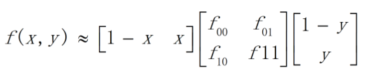
其中,双线性插值公式为:
3,加入旋转不变性
# 在圆形选取框基础上,加入旋转不变操作

def rotation_invariant_LBP(img, radius=3, neighbors=8):

    h,w=img.shape

    dst = np.zeros((h-2*radius, w-2*radius),dtype=img.dtype)

    for i in range(radius,h-radius):

        for j in range(radius,w-radius):

            # 获得中心像素点的灰度值

            center = img[i,j]

            for k in range(neighbors):

                # 计算采样点对于中心点坐标的偏移量rx,ry

                rx = radius * np.cos(2.0 * np.pi * k / neighbors)

                ry = -(radius * np.sin(2.0 * np.pi * k / neighbors))

                # 为双线性插值做准备

                # 对采样点偏移量分别进行上下取整

                x1 = int(np.floor(rx))

                x2 = int(np.ceil(rx))

                y1 = int(np.floor(ry))

                y2 = int(np.ceil(ry))

                # 将坐标偏移量映射到0-1之间

                tx = rx - x1

                ty = ry - y1

                # 根据0-1之间的x,y的权重计算公式计算权重,权重与坐标具体位置无关,与坐标间的差值有关

                w1 = (1-tx) * (1-ty)

                w2 =    tx  * (1-ty)

                w3 = (1-tx) *    ty

                w4 =    tx  *    ty

                # 根据双线性插值公式计算第k个采样点的灰度值

                neighbor = img[i+y1,j+x1] * w1 + img[i+y2,j+x1] *w2 + img[i+y1,j+x2] *  w3 +img[i+y2,j+x2] *w4

                # LBP特征图像的每个邻居的LBP值累加,累加通过与操作完成,对应的LBP值通过移位取得

                dst[i-radius,j-radius] |= (neighbor>center)  <<  (np.uint8)(neighbors-k-1)

    # 进行旋转不变处理

    for i in range(dst.shape[0]):

        for j in range(dst.shape[1]):

            currentValue = dst[i,j]

            minValue = currentValue

            for k in range(1, neighbors):

                # 对二进制编码进行循环左移,意思即选取移动过程中二进制码最小的那个作为最终值

                temp = (np.uint8)(currentValue>>(neighbors-k)) |  (np.uint8)(currentValue<<k)

                if temp < minValue:

                    minValue = temp

            dst[i,j] = minValue

    return dst

gray = cv2.imread(image_path, cv2.IMREAD_GRAYSCALE)

rotation_invariant = rotation_invariant_LBP(gray,3,8)

cv2.imshow('img', gray)

cv2.imshow('ri', rotation_invariant)

cv2.waitKey(0)

cv2.destroyAllWindows()
4,等价模式
def get_shifts(data):

    '''

    计算跳变次数,即二进制码相邻2位不同,总共出现的次数

    '''

    count = 0

    binaryCode = "{0:0>8b}".format(data)

    for i in range(1,len(binaryCode)):

        if binaryCode[i] != binaryCode[(i-1)]:

            count+=1

    return count

def create_table(img):

    # LBP特征值对应图像灰度编码表,直接默认采样点为8位

    temp = 1

    table =np.zeros((256),dtype=img.dtype)

    for i in range(256):

#         跳变小于3定义为等价模式类,共58,混合类算做1种

        if get_shifts(i)<3:

            table[i] = temp

            temp+=1

    return table

# 等价模式类:二进制码跳变次数小于3,8位二进制码共58种等价模式,其他256-58种为混合类。混合类的LBP特征将置为0,所以最终图像偏暗

def uniform_pattern_LBP(img,table,radius=3, neighbors=8):

    h,w=img.shape

    dst = np.zeros((h-2*radius, w-2*radius),dtype=img.dtype)

    for i in range(radius,h-radius):

        for j in range(radius,w-radius):

            # 获得中心像素点的灰度值

            center = img[i,j]

            for k in range(neighbors):

                # 计算采样点对于中心点坐标的偏移量rx,ry

                rx = radius * np.cos(2.0 * np.pi * k / neighbors)

                ry = -(radius * np.sin(2.0 * np.pi * k / neighbors))

                # 为双线性插值做准备

                # 对采样点偏移量分别进行上下取整

                x1 = int(np.floor(rx))

                x2 = int(np.ceil(rx))

                y1 = int(np.floor(ry))

                y2 = int(np.ceil(ry))

                # 将坐标偏移量映射到0-1之间

                tx = rx - x1

                ty = ry - y1

                # 根据0-1之间的x,y的权重计算公式计算权重,权重与坐标具体位置无关,与坐标间的差值有关

                w1 = (1-tx) * (1-ty)

                w2 =    tx  * (1-ty)

                w3 = (1-tx) *    ty

                w4 =    tx  *    ty

                # 根据双线性插值公式计算第k个采样点的灰度值

                neighbor = img[i+y1,j+x1] * w1 + img[i+y2,j+x1] *w2 + img[i+y1,j+x2] *  w3 +img[i+y2,j+x2] *w4

                # LBP特征图像的每个邻居的LBP值累加,累加通过与操作完成,对应的LBP值通过移位取得

                dst[i-radius,j-radius] |= (neighbor>center)  <<  (np.uint8)(neighbors-k-1)

                # 进行LBP特征的UniformPattern编码

                # 8位二进制码形成后,查表,对属于混合类的特征置0

                if k==neighbors-1:

                    dst[i-radius,j-radius] = table[dst[i-radius,j-radius]]

    return dst

gray = cv2.imread(image_path, cv2.IMREAD_GRAYSCALE)

table=create_table(gray)

uniform_pattern = uniform_pattern_LBP(gray,table,3,8)

cv2.imshow('img', gray)

cv2.imshow('up', uniform_pattern)

cv2.waitKey(0)

cv2.destroyAllWindows()
5,MB_LBP:先对像素做区域平均处理,再使用原始LBP
# 先对像素分割,用一个小区域的平均值代替这个区域,再用LBP特征处理

def multi_scale_block_LBP(img,scale):

    h,w= img.shape

    # cellSize表示一个cell大小

    cellSize = int(scale / 3)

    offset = int(cellSize / 2)

    cellImage = np.zeros((h-2*offset, w-2*offset),dtype=img.dtype)

    for i in range(offset,h-offset):

        for j in range(offset,w-offset):

            temp = 0

            for m in range(-offset,offset+1):

                for n in range(-offset,offset+1):

                    temp += img[i+n,j+m]

#             即取一个cell里所有像素的平均值

            temp /= (cellSize*cellSize)

            cellImage[i-offset,j-offset] = np.uint8(temp)

#     再对平均后的像素做LBP特征处理

    dst = origin_LBP(cellImage)

    return dst

gray = cv2.imread(image_path, cv2.IMREAD_GRAYSCALE)

mb_3 = multi_scale_block_LBP(gray,3)

mb_9 = multi_scale_block_LBP(gray,9)

mb_15 = multi_scale_block_LBP(gray,15)

cv2.imshow('img', gray)

cv2.imshow('mb_3', mb_3)

cv2.imshow('mb_9', mb_9)

cv2.imshow('mb_15', mb_15)

cv2.waitKey(0)

cv2.destroyAllWindows()
5,LBPH,Local Binary Patterns Histograms
此处基于等价模式,再使用像素各分割块的直方统计图,拼接为最后的特征向量
# 先使用等价模式预处理图像,降维。再分割图像,对每个分割块进行直方统计(降维后的类别为59),返回密度向量,再拼接各个分割块对应的密度向量

# 最终返回grid_x*grid_y*numPatterns维的特征向量,作为图像的LBPH特征向量

def getLBPH(img_lbp,numPatterns,grid_x,grid_y,density):

    '''

    计算LBP特征图像的直方图LBPH

    '''

    h,w=img_lbp.shape

    width = int(w / grid_x)

    height = int(h / grid_y)

    # 定义LBPH的行和列,grid_x*grid_y表示将图像分割的块数,numPatterns表示LBP值的模式种类

    result = np.zeros((grid_x * grid_y,numPatterns),dtype=float)

    resultRowIndex = 0

    # 对图像进行分割,分割成grid_x*grid_y块,grid_x,grid_y默认为8

    for i in range(grid_x):

        for j in range(grid_y):

            # 图像分块

            src_cell = img_lbp[i*height:(i+1)*height,j*width:(j+1)*width]

            # 计算直方图

            hist_cell = getLocalRegionLBPH(src_cell,0,(numPatterns-1),density)

            #将直方图放到result中

            result[resultRowIndex]=hist_cell

            resultRowIndex+=1

    return np.reshape(result,(-1))

def getLocalRegionLBPH(src,minValue,maxValue,density=True):

    '''

    计算一个LBP特征图像块的直方图

    '''

    data = np.reshape(src,(-1))

    # 计算得到直方图bin的数目,直方图数组的大小

    bins = maxValue - minValue + 1;

    # 定义直方图每一维的bin的变化范围

    ranges = (float(minValue),float(maxValue + 1))

#     density为True返回的是每个bin对应的概率值,bin为单位宽度时,概率总和为1

    hist, bin_edges = np.histogram(src, bins=bins, range=ranges, density=density)

    return hist

uniform_pattern = uniform_pattern_LBP(gray,table,3,8)

#等价模式58种,混合模式算1种

lbph = getLBPH(uniform_pattern,59,8,8,True)
参考博客:https://blog.csdn.net/lk3030/article/details/84034963
Opencv之LBP特征(算法)的更多相关文章
- OpenCV开发笔记(五十五):红胖子8分钟带你深入了解Haar、LBP特征以及级联分类器识别过程(图文并茂+浅显易懂+程序源码)
若该文为原创文章,未经允许不得转载原博主博客地址:https://blog.csdn.net/qq21497936原博主博客导航:https://blog.csdn.net/qq21497936/ar ...
- 行人检测4(LBP特征)
参考原文: http://blog.csdn.net/zouxy09/article/details/7929531 http://www.cnblogs.com/dwdxdy/archive/201 ...
- 图像物体检測识别中的LBP特征
版权声明:本文为博主原创文章,未经博主同意不得转载. https://blog.csdn.net/xinzhangyanxiang/article/details/37317863 图像物体检測识别中 ...
- LBP特征
此篇摘取 <LBP特征原理及代码实现> <LBP特征 学习笔记> 另可参考实现: <LBP特征学习及实现> <LBP特征的实现及LBP+SVM分类> & ...
- 图像的全局特征--LBP特征
原文链接:http://blog.csdn.net/zouxy09/article/details/7929531#comments 这个特征或许对三维图像特征提取有很大作用.文章有修改,如有疑问,请 ...
- OpenCV人脸识别LBPH算法源码分析
1 背景及理论基础 人脸识别是指将一个需要识别的人脸和人脸库中的某个人脸对应起来(类似于指纹识别),目的是完成识别功能,该术语需要和人脸检测进行区分,人脸检测是在一张图片中把人脸定位出来,完成的是搜寻 ...
- OpenCV 轮廓基本特征
http://blog.csdn.net/tiemaxiaosu/article/details/51360499 OpenCV 轮廓基本特征 2016-05-10 10:26 556人阅读 评论( ...
- 图像特征提取之LBP特征
LBP(Local Binary Pattern,局部二值模式)是一种用来描述图像局部纹理特征的算子:它具有旋转不变性和灰度不变性等显著的优点.它是首先由T. Ojala, M.Pietik?inen ...
- 图像特征提取三大法宝:HOG特征,LBP特征,Haar特征(转载)
(一)HOG特征 1.HOG特征: 方向梯度直方图(Histogram of Oriented Gradient, HOG)特征是一种在计算机视觉和图像处理中用来进行物体检测的特征描述子.它通过计算和 ...
随机推荐
- Java分级考试
石家庄铁道大学选课管理系统 1.项目需求: 本项目所开发的学生选课系统完成学校对学生的选课信息的统计与管理,减少数据漏掉的情况,同时也节约人力.物力和财力.告别以往的人工统计. 2.系统要求与功能设计 ...
- Python CGI编程Ⅵ
GET和POST方法 浏览器客户端通过两种方法向服务器传递信息,这两种方法就是 GET 方法和 POST 方法. 使用GET方法传输数据 GET方法发送编码后的用户信息到服务端,数据信息包含在请求页面 ...
- jquery keydown()方法 语法
jquery keydown()方法 语法 作用:完整的 key press 过程分为两个部分:1. 按键被按下:2. 按键被松开.当按钮被按下时,发生 keydown 事件.keydown() 方法 ...
- Ubuntu镜像的MD5校验
造冰箱的大熊猫@cnblogs 2018/9/7 1.在Ubuntu终端中,按照以下格式输入命令计算镜像文件ubuntu-xxx.iso的MD5校验和. md5sum ubuntu-xxx.iso 2 ...
- javascript中的原型和原型链(一)
原型和原型链是 JS 中不可避免需要碰到的知识点,本文使用图片思维导图的形式缕一缕原型.原型链.实例.构造函数等等概念之间的关系. Constructor 构造函数 首先我们先写一个构造函数 Pers ...
- Confluence 6 多媒体文件和在页面中显示文件列表
多媒体文件 文件的预览同时也支持 MP3 音频和 MP4 视频文件.Confluence 使用 HTML 5 来播放附加的音频和视频文件.这个意味着这些文件类型的文件格式,用户可以在支持的浏览器中直接 ...
- sh_10_字典基本使用
sh_10_字典基本使用 xiaoming_dict = {"name": "小明"} # 1. 取值 print(xiaoming_dict["na ...
- Unity3D_(数据)JsonUtility创建和解析Json
Json 百度百科:传送门 LitJson创建和解析Json 传送门 Json数据解析在Unity3d中的应用 传送门 一.使用JsonUnity创建Json using System.Collect ...
- C++入门经典-例3.24-找图书的位置
1:运行代码: // 3.24.cpp : 定义控制台应用程序的入口点. // #include "stdafx.h" #include <iostream> usin ...
- MySQL 数据库 常用函数
一.数学函数 数学函数主要用于处理数字,包括整型.浮点数等. ABS(x) 返回x的绝对值 SELECT ABS(-1) -- 返回1 CEIL(x),CEILING(x) 返回大于或等于x的最小整数 ...