2. Spark GraphX解析

2.1 存储模式

　　2.1.1 图存储模式

　　　　　　巨型图的存储总体上有边分割和点分割两种存储方式

　　　　　　1）边分割(Edge-Cut)：每个顶点都存储一次，但有的边会被打断分到两台机器上。这样做的好处是节省存储空间；坏处是对图进行基于边的计算时，对于一条两个顶点被分到不同机器上的边来说，要跨机器通信传输数据，内网通信流量大

　　　　　　2）点分割(Vertex-Cut)：每条边只存储一次，都只会出现在一台机器上。邻居多的点会被复制到多台机器上，增加了存储开销，同时会引发数据同步问题。好处是可以大幅减少内网通信量

　　　　　　虽然两种方法互有利弊，但现在是点分割占上风，各种分布式图计算框架都将自己底层的存储形式变成了点分割

　　　　　　1）磁盘价格下降，存储空间不再是问题，而内网的通信资源没有突破性进展，集群计算时内网带宽是宝贵的，时间比磁盘更珍贵。这点就类似于常见的空间换时间的策略

　　　　　　2）在当前的应用场景中，绝大多数网络都是“无尺度网络”，遵循幂律分布，不同点的邻居数量相差非常悬殊。而边分割会使那些多邻居的点所相连的边大多数被分到不同的机器上，这样的数据分布会使得内网带宽更加捉襟见肘，于是边分割存储方式被渐渐抛弃了

　　2.1.2 GraphX存储模式

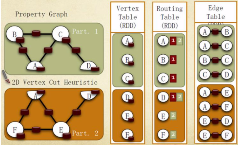
　　　　　　Graphx借鉴PowerGraph，使用的是Vertex-Cut(点分割)方式存储图，用三个RDD存储图数据信息

　　　　　　VertexTable(id, data)：id为顶点id，data为顶点属性

　　　　　　EdgeTable(pid, src, dst, data)：pid为分区id，src为源顶点id，dst为目的顶点id，data为边属性

　　　　　　RoutingTable(id, pid)：id为顶点id，pid为分区id

　　　　　　点分割存储实现如下图所示：

　　　　　　

　　　　　　GraphX在进行图分割时，有几种不同的分区(partition)策略，它通过PartitionStrategy专门定义这些策略。在PartitionStrategy中，总共定义了EdgePartition2D、EdgePartition1D、RandomVertexCut以及CanonicalRandomVertexCut这四种不同的分区策略。下面分别介绍这几种策略

　　2.1.2.1 RandomVertexCut

case object RandomVertexCut extends PartitionStrategy {
  override def getPartition(src: VertexId, dst: VertexId, numParts:
  PartitionID): PartitionID = {
    math.abs((src, dst).hashCode()) % numParts
  }
}

　　　　　　这个方法比较简单，通过取源顶点和目标顶点id的哈希值来将边分配到不同的分区。这个方法会产生一个随机的边分割，两个顶点之间相同方向的边会分配到同一个分区

　　2.1.2.2 CanonicalRandomVertexCut

case object CanonicalRandomVertexCut extends PartitionStrategy {
  override def getPartition(src: VertexId, dst: VertexId, numParts:
PartitionID): PartitionID = {
    if (src < dst) {
      math.abs((src, dst).hashCode()) % numParts
    } else {
      math.abs((dst, src).hashCode()) % numParts
    }
  }
}

　　　　　　这种分割方法和前一种方法没有本质的不同。不同的是，哈希值的产生带有确定的方向(即两个顶点中较小的id的顶点在前)。两个顶点之间所有的边都会分配到同一个分区，而不管方向如何

　　2.1.2.3 EdgePartition1D　　

case object EdgePartition1D extends PartitionStrategy {
  override def getPartition(src: VertexId, dst: VertexId, numParts:
  PartitionID): PartitionID = {
    val mixingPrime: VertexId = 1125899906842597L (math.abs(src * mixingPrime) % numParts).toInt
  }
}

　　　　　　这种方法仅仅根据源顶点id来将边分配到不同的分区。有相同源顶点的边会分配到同一分区

　　2.1.2.4 EdgePartition2D

case object EdgePartition2D extends PartitionStrategy {
  override def getPartition(src: VertexId, dst: VertexId, numParts:
  PartitionID): PartitionID = {
    val ceilSqrtNumParts: PartitionID = math.ceil(math.sqrt(numParts)).toInt
    val mixingPrime: VertexId = 1125899906842597L
    if (numParts == ceilSqrtNumParts * ceilSqrtNumParts) {
      // Use old method for perfect squared to ensure we get same results
      val col: PartitionID = (math.abs(src * mixingPrime) %
        ceilSqrtNumParts).toInt
      val row: PartitionID = (math.abs(dst * mixingPrime) %
        ceilSqrtNumParts).toInt
      (col * ceilSqrtNumParts + row) % numParts
    } else {
      // Otherwise use new method
      val cols = ceilSqrtNumParts
      val rows = (numParts + cols - 1) / cols
      val lastColRows = numParts - rows * (cols - 1)
      val col = (math.abs(src * mixingPrime) % numParts / rows).toInt
      val row = (math.abs(dst * mixingPrime) % (
        if (col < cols - 1)
          rows
        else
          lastColRows)).toInt
      col * rows + row
    }
  }
}

　　　　　　这种分割方法同时使用到了源顶点id和目的顶点id。它使用稀疏边连接矩阵的2维区分来将边分配到不同的分区，从而保证顶点的备份数不大于2 * sqrt(numParts)的限制。这里numParts表示分区数。这个方法的实现分两种情况，即分区数能完全开方和不能完全开方两种情况。当分区数能完全开方时，采用下面的方法：

val col: PartitionID = (math.abs(src * mixingPrime) % ceilSqrtNumParts).toInt
val row: PartitionID = (math.abs(dst * mixingPrime) % ceilSqrtNumParts).toInt
(col * ceilSqrtNumParts + row) % numParts

　　　　　　当分区数不能完全开方时，采用下面的方法。这个方法的最后一列允许拥有不同的行数　

val cols = ceilSqrtNumParts
val rows = (numParts + cols - 1) / cols
//最后一列允许不同的行数
val lastColRows = numParts - rows * (cols - 1)
val col = (math.abs(src * mixingPrime) % numParts / rows).toInt
val row = (math.abs(dst * mixingPrime) % (
  if (col < cols - 1)
    rows
  else
    lastColRows)
  ).toInt
col * rows + row

　　　　　　下面举个例子来说明该方法。假设我们有一个拥有12个顶点的图，要把它切分到9台机器。我们可以用下面的稀疏矩阵来表示：

　　　　　　

　　　　　　上面的例子中*表示分配到处理器上的边。E表示连接顶点v11和v1的边，它被分配到了处理器P6上。为了获得边所在的处理器，我们将矩阵切分为sqrt(numParts) * sqrt(numParts)块。注意，上图中与顶点v11相连接的边只出现在第一列的块(P0,P3,P6)或者最后一行的块(P6,P7,P8)中，这保证了V11的副本数不会超过2*sqrt(numParts)份，在上例中即副本不能超过6份。

　　　　　　在上面的例子中，P0里面存在很多边，这会造成工作的不均衡。为了提高均衡，我们首先用顶点id乘以一个大的素数，然后再shuffle顶点的位置。乘以一个大的素数本质上不能解决不平衡的问题，只是减少了不平衡的情况发生

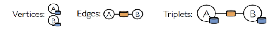
2.2 vertices、edges以及triplets

　　　　　　vertices、edges 以及 triplets 是 GraphX 中三个非常重要的概念，在前文GraphX介绍中对这三个概念有初步的了解

　　2.2.1 vertices

　　　　　　在GraphX中，vertices对应着名称为VertexRDD的RDD。这个RDD有顶点id和顶点属性两个成员变量。它的源码如下所示：

abstract class VertexRDD[VD](sc: SparkContext, deps: Seq[Dependency[_]]) extends RDD[(VertexId, VD)](sc, deps)

　　　　　　从源码中我们可以看到，VertexRDD继承自RDD[(VertexId, VD)]，这里VertexId表示顶点id，VD表示顶点所带的属性的类别。这从另一个角度也说明VertexRDD拥有顶点id和顶点属性

　　2.2.2 edges

　　　　　　在GraphX中，edges对应着EdgeRDD。这个RDD拥有三个成员变量，分别是源顶点id、目标顶点id以及边属性。它的源码如下所示：

abstract class EdgeRDD[ED](sc: SparkContext, deps: Seq[Dependency[_]]) extends RDD[Edge[ED]](sc, deps)

　　　　　　从源码中可以看到，EdgeRDD继承自RDD[Edge[ED]]，即类型为Edge[ED]的RDD

　　2.2.3 triplets

　　　　　　在GraphX中，triplets对应着EdgeTriplet。它是一个三元组视图，这个视图逻辑上将顶点和边的属性保存为一个RDD[EdgeTriplet[VD, ED]]。可以通过下面的Sql表达式表示这个三元视图的含义：

SELECT
      src.id,
      dst.id,
      src.attr,
      e.attr,
      dst.attr
FROM
      edges AS e
LEFT JOIN vertices AS src,
  vertices AS dst ON e.srcId = src.Id
AND e.dstId = dst.Id

　　　　　　同样，也可以通过下面的图解的形式来表示它的含义：

　　　　　　

　　　　　　EdgeTriplet的源代码如下所示：

class EdgeTriplet[VD, ED] extends Edge[ED] {
  //源顶点属性
  var srcAttr: VD = _ // nullValue[VD]
  //目标顶点属性
  var dstAttr: VD = _ // nullValue[VD]
  protected[spark] def set(other: Edge[ED]): EdgeTriplet[VD, ED] = {
    srcId = other.srcId
    dstId = other.dstId
    attr = other.attr
    this
  }
}

　　　　　　EdgeTriplet 类继承自 Edge 类，我们来看看这个父类：

case class Edge[@specialized(Char, Int, Boolean, Byte, Long, Float, Double) ED] (var srcId: VertexId = 0, var dstId: VertexId = 0, var attr: ED = null.asInstanceOf[ED]) extends Serializable

　　　　　　Edge类中包含源顶点id，目标顶点id以及边的属性。所以从源代码中我们可以知道，triplets既包含了边属性也包含了源顶点的id和属性、目标顶点的id和属性

2.3 图的构建

　　　　　　GraphX的Graph对象是用户操作图的入口。前面的章节我们介绍过，它包含了边(edges)、顶点(vertices)以及triplets三部分，并且这三部分都包含相应的属性，可以携带额外的信息

　　2.3.1 构建图的方法

　　　　　　构建图的入口方法有两种，分别是根据边构建和根据边的两个顶点构建

　　2.3.1.1 根据边构建图(Graph.fromEdges)

def fromEdges[VD: ClassTag, ED: ClassTag](
  edges: RDD[Edge[ED]],
  defaultValue: VD,
  edgeStorageLevel: StorageLevel = StorageLevel.MEMORY_ONLY, vertexStorageLevel: StorageLevel = StorageLevel.MEMORY_ONLY): Graph[VD,
  ED] = {
  GraphImpl(edges, defaultValue, edgeStorageLevel, vertexStorageLevel)
}

　　2.3.1.2 根据边的两个顶点数据构建(Graph.fromEdgeTuples)

def fromEdgeTuples[VD: ClassTag](
    rawEdges: RDD[(VertexId, VertexId)],
    defaultValue: VD,
    uniqueEdges: Option[PartitionStrategy] = None,
    edgeStorageLevel: StorageLevel = StorageLevel.MEMORY_ONLY, vertexStorageLevel: StorageLevel = StorageLevel.MEMORY_ONLY): Graph[VD,
    Int] = {
  val edges = rawEdges.map(p => Edge(p._1, p._2, 1))
  val graph = GraphImpl(edges, defaultValue, edgeStorageLevel, vertexStorageLevel)
  uniqueEdges match {
    case Some(p) => graph.partitionBy(p).groupEdges((a, b) => a + b)
    case None => graph
  }
}

　　　　　　从上面的代码我们知道，不管是根据边构建图还是根据边的两个顶点数据构建，最终都是使用GraphImpl来构建的，即调用了GraphImpl的apply方法

　　2.3.2 构建图的过程

　　　　　　构建图的过程很简单，分为三步，它们分别是构建边EdgeRDD、构建顶点VertexRDD、生成Graph对象。下面分别介绍这三个步骤

2.3.2.1 构建边EdgeRDD也分为三步，下图的例子详细说明了这些步骤

　　　　　　

　　　　　　1 从文件中加载信息，转换成tuple的形式，即(srcId，dstId)

val rawEdgesRdd: RDD[(Long, Long)] =
  sc.textFile(input).filter(s => s != "0,0").repartition(partitionNum).map {
  case line =>
    val ss = line.split(",")
    val src = ss(0).toLong
    val dst = ss(1).toLong
    if (src < dst)
      (src, dst)
    else
      (dst, src)
}.distinct()

　　　　　　2 入口，调用Graph.fromEdgeTuples(rawEdgesRdd)

　　　　　　源数据为分割的两个点ID，把源数据映射成Edge(srcId, dstId, attr)对象, attr默认为1。这样元数据就构建成了RDD[Edge[ED]]，如下面的代码

val edges = rawEdges.map(p => Edge(p._1, p._2, 1))

　　　　　　3 将RDD[Edge[ED]]进一步转化成EdgeRDDImpl[ED，VD]

　　　　　　第二步构建完RDD[Edge[ED]]之后，GraphX通过调用GraphImpl的apply方法来构建Graph

val graph = GraphImpl(edges, defaultValue, edgeStorageLevel,
  vertexStorageLevel)
  def apply[VD: ClassTag, ED: ClassTag](
        edges: RDD[Edge[ED]],
        defaultVertexAttr: VD,
        edgeStorageLevel: StorageLevel,
        vertexStorageLevel: StorageLevel): GraphImpl[VD, ED] = {
  fromEdgeRDD(EdgeRDD.fromEdges(edges), defaultVertexAttr, edgeStorageLevel, vertexStorageLevel)
}

　　　　　　在apply调用fromEdgeRDD之前，代码会调用EdgeRDD.fromEdges(edges)将RDD[Edge[ED]]转化成 EdgeRDDImpl[ED, VD]

def fromEdges[ED: ClassTag, VD: ClassTag](edges: RDD[Edge[ED]]): EdgeRDDImpl[ED, VD] = {
  val edgePartitions = edges.mapPartitionsWithIndex { (pid, iter) =>
    val builder = new EdgePartitionBuilder[ED, VD]
    iter.foreach { e =>
      builder.add(e.srcId, e.dstId, e.attr)
    }
    Iterator((pid, builder.toEdgePartition))
  }
  EdgeRDD.fromEdgePartitions(edgePartitions)
}

　　　　　　程序遍历RDD[Edge[ED]]的每个分区，并调用builder.toEdgePartition对分区内的边作相应的处理

def toEdgePartition: EdgePartition[ED, VD] = {
  val edgeArray = edges.trim().array
  new Sorter(Edge.edgeArraySortDataFormat[ED])
    .sort(edgeArray, 0, edgeArray.length, Edge.lexicographicOrdering)
  val localSrcIds = new Array[Int](edgeArray.size)
  val localDstIds = new Array[Int](edgeArray.size)
  val data = new Array[ED](edgeArray.size)
  val index = new GraphXPrimitiveKeyOpenHashMap[VertexId, Int]
  val global2local = new GraphXPrimitiveKeyOpenHashMap[VertexId, Int]
  val local2global = new PrimitiveVector[VertexId]
  var vertexAttrs = Array.empty[VD]
  //采用列式存储的方式，节省了空间
  if (edgeArray.length > 0) {
    index.update(edgeArray(0).srcId, 0)
    var currSrcId: VertexId = edgeArray(0).srcId var currLocalId = -1
    var i = 0
    while (i < edgeArray.size) {
      val srcId = edgeArray(i).srcId
      val dstId = edgeArray(i).dstId
      localSrcIds(i) = global2local.changeValue(srcId,
      { currLocalId += 1; local2global += srcId; currLocalId }, identity) localDstIds(i) = global2local.changeValue(dstId,
      { currLocalId += 1; local2global += dstId; currLocalId }, identity)
      data(i) = edgeArray(i).attr
      //相同顶点 srcId 中第一个出现的 srcId 与其下标
      if (srcId != currSrcId) {
        currSrcId = srcId
        index.update(currSrcId, i)
      }
      i += 1
    }
    vertexAttrs = new Array[VD](currLocalId + 1)
  }
  new EdgePartition(
  localSrcIds, localDstIds, data, index, global2local,
  local2global.trim().array, vertexAttrs, None)
}

　　　　　　toEdgePartition的第一步就是对边进行排序

　　　　　　　　按照srcId从小到大排序。排序是为了遍历时顺序访问，加快访问速度。采用数组而不是Map，是因为数组是连续的内存单元，具有原子性，避免了Map的hash 问题，访问速度快

　　　　　　toEdgePartition的第二步就是填充localSrcIds，localDstIds，data，index，global2local，local2global，vertexAttrs

　　　　　　　　数组localSrcIds，localDstIds中保存的是通过global2local.changeValue(srcId/dstId)转换而成的分区本地索引。可以通过localSrcIds、localDstIds数组中保存的索引位从local2global中查到具体的VertexId

　　　　　　　　global2local是一个简单的，key值非负的快速hash map:GraphXPrimitiveKeyOpenHashMap, 保存vertextId和本地索引的映射关系。global2local中包含当前partition所有srcId、dstId与本地索引的映射关系

　　　　　　　　data就是当前分区的attr属性数组

　　　　　　　　我们知道相同的srcId可能对应不同的dstId。按照srcId排序之后，相同的srcId会出现多行，如上图中的index desc部分。index中记录的是相同srcId中第一个出现的srcId与其下标

　　　　　　　　local2global记录的是所有的VertexId信息的数组。形如: srcId,dstId,srcId,dstId,srcId,dstId,srcId,dstId。其中会包含相同的srcId。即:当前分区所有vertextId的顺序实际值

　　　　　　　　我们可以通过根据本地下标取VertexId，也可以根据VertexId取本地下标，取相应的属性

// 根据本地下标取VertexId
localSrcIds/localDstIds -> index -> local2global -> VertexId
// 根据 VertexId 取本地下标，取属性
VertexId -> global2local -> index -> data -> attr object

　　2.3.2.2 构建顶点VertexRDD

　　　　　　紧接着上面构建边RDD的代码，方法fromEdgeRDD的实现

private def fromEdgeRDD[VD: ClassTag, ED: ClassTag](
        edges: EdgeRDDImpl[ED, VD],
        defaultVertexAttr: VD,
        edgeStorageLevel: StorageLevel,
        vertexStorageLevel: StorageLevel): GraphImpl[VD, ED] = {
  val edgesCached = edges.withTargetStorageLevel(edgeStorageLevel).cache()
  val vertices = VertexRDD.fromEdges(edgesCached, edgesCached.partitions.size, defaultVertexAttr)
  .withTargetStorageLevel(vertexStorageLevel)
  fromExistingRDDs(vertices, edgesCached)
}

　　　　　　从上面的代码我们可以知道，GraphX使用VertexRDD.fromEdges构建顶点VertexRDD，当然我们把边RDD作为参数传入

def fromEdges[VD: ClassTag](edges: EdgeRDD[_], numPartitions: Int, defaultVal: VD): VertexRDD[VD] = {
  //1 创建路由表
  val routingTables = createRoutingTables(edges, new HashPartitioner(numPartitions))
  //2 根据路由表生成分区对象vertexPartitions
  val vertexPartitions = routingTables.mapPartitions({ routingTableIter =>
    val routingTable =
      if (routingTableIter.hasNext)
        routingTableIter.next()
      else
        RoutingTablePartition.empty
    Iterator(ShippableVertexPartition(Iterator.empty, routingTable, defaultVal))
  }, preservesPartitioning = true)
  //3 创建 VertexRDDImpl 对象
  new VertexRDDImpl(vertexPartitions)
}

　　　　　　构建顶点VertexRDD的过程分为三步，如上代码中的注释。它的构建过程如下图所示：

　　　　　　

　　　　　　创建路由表

　　　　　　　　为了能通过点找到边，每个点需要保存点到边的信息，这些信息保存在RoutingTablePartition中

private[graphx] def createRoutingTables(edges: EdgeRDD[_], vertexPartitioner: Partitioner): RDD[RoutingTablePartition] = {
  // 将 edge partition 中的数据转换成 RoutingTableMessage 类型，
  val vid2pid = edges.partitionsRDD.mapPartitions(_.flatMap(
    Function.tupled(RoutingTablePartition.edgePartitionToMsgs)))
}

　　　　　　　　上述程序首先将边分区中的数据转换成RoutingTableMessage 类型，即tuple(VertexId,Int)类型

def edgePartitionToMsgs(pid: PartitionID, edgePartition: EdgePartition[_, _]): Iterator[RoutingTableMessage] = {

  val map = new GraphXPrimitiveKeyOpenHashMap[VertexId, Byte]
  edgePartition.iterator.foreach { e =>
    map.changeValue(e.srcId, 0x1, (b: Byte) => (b | 0x1).toByte)
    map.changeValue(e.dstId, 0x2, (b: Byte) => (b | 0x2).toByte)
  }
  map.iterator.map { vidAndPosition =>
    val vid = vidAndPosition._1
    val position = vidAndPosition._2
    toMessage(vid, pid, position)
  }
}
  //`30-0`比特位表示边分区`ID`,`32-31`比特位表示标志位
private def toMessage(vid: VertexId, pid: PartitionID, position: Byte): RoutingTableMessage = {
  val positionUpper2 = position << 30
  val pidLower30 = pid & 0x3FFFFFFF
  (vid, positionUpper2 | pidLower30)
}

　　　　　　　　根据代码，可以知道程序使用int的32-31比特位表示标志位，即01: isSrcId ,10: isDstId。30-0比特位表示边分区ID。这样做可以节省内存RoutingTableMessage表达的信息是:顶点id和它相关联的边的分区id是放在一起的，所以任何时候，我们都可以通过RoutingTableMessage找到顶点关联的边

　　　　　　根据路由表生成分区对象

private[graphx] def createRoutingTables(
  edges: EdgeRDD[_], vertexPartitioner:
  Partitioner): RDD[RoutingTablePartition] = {
  // 将 edge partition 中的数据转换成 RoutingTableMessage 类型，
  val numEdgePartitions = edges.partitions.size
  vid2pid.partitionBy(vertexPartitioner).mapPartitions(
  iter => Iterator(RoutingTablePartition.fromMsgs(numEdgePartitions, iter)),
  preservesPartitioning = true)
}

　　　　　　我们将第1步生成的vid2pid按照HashPartitioner重新分区。我们看看RoutingTablePartition.fromMsgs方法

def fromMsgs(numEdgePartitions: Int, iter: Iterator[RoutingTableMessage]): RoutingTablePartition = {

  val pid2vid = Array.fill(numEdgePartitions)(new PrimitiveVector[VertexId])
  val srcFlags = Array.fill(numEdgePartitions)(new PrimitiveVector[Boolean])
  val dstFlags = Array.fill(numEdgePartitions)(new PrimitiveVector[Boolean])
  for(msg <- iter){
    val vid = vidFromMessage(msg)
    val pid = pidFromMessage(msg)
    val position = positionFromMessage(msg)
    pid2vid(pid) += vid
    srcFlags(pid) += (position & 0x1) != 0
    dstFlags(pid) += (position & 0x2) != 0
  }
  new RoutingTablePartition(pid2vid.zipWithIndex.map{
    case (vids, pid) => (vids.trim().array, toBitSet(srcFlags(pid) ), toBitSet(dstFlags(pid)))
  })
}

　　　　　　该方法从RoutingTableMessage获取数据，将vid, 边pid, isSrcId/isDstId重新封装到pid2vid，srcFlags，dstFlags这三个数据结构中。它们表示当前顶点分区中的点在边分区的分布。想象一下，重新分区后，新分区中的点可能来自于不同的边分区，所以一个点要找到边，就需要先确定边的分区号pid，然后在确定的边分区中确定是srcId还是 dstId, 这样就找到了边。新分区中保存vids.trim().array, toBitSet(srcFlags(pid)), toBitSet(dstFlags(pid))这样的记录。这里转换为toBitSet保存是为了节省空间

　　　　　　根据上文生成的routingTables，重新封装路由表里的数据结构为ShippableVertexPartition。ShippableVertexPartition会合并相同重复点的属性attr对象，补全缺失的attr对象

def apply[VD: ClassTag](
  iter: Iterator[(VertexId, VD)], routingTable: RoutingTablePartition, defaultVal: VD,
  mergeFunc: (VD, VD) => VD): ShippableVertexPartition[VD] =
{
  val map = new GraphXPrimitiveKeyOpenHashMap[VertexId, VD]
  // 合并顶点
  iter.foreach{ pair =>
  map.setMerge(pair._1, pair._2, mergeFunc)}
  // 不全缺失的属性值
  routingTable.iterator.foreach{ vid =>
    map.changeValue(vid, defaultVal, identity)
  }
  new ShippableVertexPartition(map.keySet, map._values, map.keySet.getBitSet, routingTable)
  //ShippableVertexPartition 定义
  ShippableVertexPartition[VD: ClassTag](
  val index: VertexIdToIndexMap,
  val values: Array[VD],
  val mask: BitSet,
  val routingTable: RoutingTablePartition)

　　　　　　map就是映射vertexId->attr，index就是顶点集合，values就是顶点集对应的属性集，mask指顶点集的BitSet

　　2.3.2.3 生成Graph对象

　　　　　　使用上述构建的edgeRDD和vertexRDD，使用new GraphImpl(vertices, new ReplicatedVertexView(edges.asInstanceOf[EdgeRDDImpl[ED, VD]]))就可以生成 Graph对象。ReplicatedVertexView是点和边的视图，用来管理运送(shipping)顶点属性到EdgeRDD的分区。当顶点属性改变时，我们需要运送它们到边分区来更新保存在边分区的顶点属性。注意，在ReplicatedVertexView中不要保存一个对边的引用，因为在属性运送等级升级后，这个引用可能会发生改变

class ReplicatedVertexView[VD: ClassTag, ED: ClassTag](var edges: EdgeRDDImpl[ED, VD], var hasSrcId: Boolean = false, var hasDstId: Boolean = false)

2.4 计算模式

　　2.4.1 BSP计算模式

　　　　　　目前基于图的并行计算框架已经有很多，比如来自Google的Pregel、来自Apache开源的图计算框架Giraph/HAMA以及最为著名的GraphLab，其中Pregel、HAMA 和Giraph都是非常类似的，都是基于BSP(Bulk Synchronous Parallell)模式。Bulk Synchronous Parallell，即整体同步并行

　　　　　　在BSP中，一次计算过程由一系列全局超步组成，每一个超步由并发计算、通信和同步三个步骤组成。同步完成，标志着这个超步的完成及下一个超步的开始。BSP 模式的准则是批量同步(bulk synchrony)，其独特之处在于超步(superstep)概念的引入。一个BSP程序同时具有水平和垂直两个方面的结构。从垂直上看，一个BSP程序由一系列串行的超步(superstep)组成，如图所示：

　　　　　　

　　　　　　从水平上看，在一个超步中，所有的进程并行执行局部计算。一个超步可分为三个阶段，如图所示：

　　　　　　

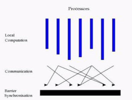
　　　　　　本地计算阶段，每个处理器只对存储在本地内存中的数据进行本地计算

　　　　　　全局通信阶段，对任何非本地数据进行操作

　　　　　　栅栏同步阶段，等待所有通信行为的结束

　　　　　　BSP模型有如下几个特点：

　　　　　　1. 将计算划分为一个一个的超步(superstep)，有效避免死锁

　　　　　　2. 将处理器和路由器分开，强调了计算任务和通信任务的分开，而路由器仅仅完成点到点的消息传递，不提供组合、复制和广播等功能，这样做既掩盖具体的互 连网络拓扑，又简化了通信协议

　　　　　　3. 采用障碍同步的方式、以硬件实现的全局同步是可控的粗粒度级，提供了执行紧耦合同步式并行算法的有效方式

　　2.4.2 图操作一览

　　　　　　正如RDDs有基本的操作map, filter和reduceByKey一样，属性图也有基本的集合操作，这些操作采用用户自定义的函数并产生包含转换特征和结构的新图。定义在 Graph中的核心操作是经过优化的实现。表示为核心操作的组合的便捷操作定义在GraphOps中。然而，因为有Scala的隐式转换，定义在GraphOps中的操作可以作为Graph的成员自动使用。例如，我们可以通过下面的方式计算每个顶点(定义在GraphOps中)的入度

val graph: Graph[(String, String), String]
// Use the implicit GraphOps.inDegrees operator
val inDegrees: VertexRDD[Int] = graph.inDegrees

　　　　　　区分核心图操作和GraphOps的原因是为了在将来支持不同的图表示。每个图表示都必须提供核心操作的实现并重用很多定义在GraphOps中的有用操作

　　　　　　

　　2.4.3 操作一览

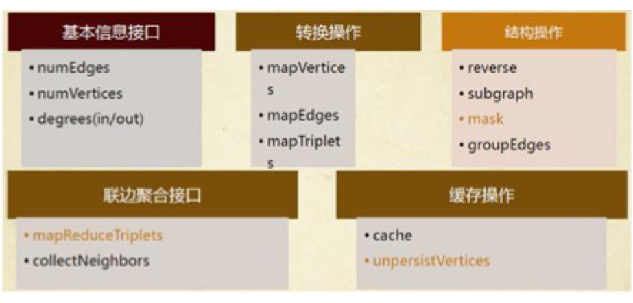
　　　　　　以下是定义在Graph和GraphOps中(为了简单起见，表现为图的成员)的功能的快速浏览。注意，某些函数签名已经简化(如默认参数和类型的限制已删除)，一些更高级的功能已经被删除，所以请参阅API文档了解官方的操作列表

　　　　　　

import org.apache.spark._
import org.apache.spark.graphx._
import org.apache.spark.rdd.RDD

val users: VertexRDD[(String, String)] = VertexRDD[(String, String)](sc.parallelize(Array((3L, ("rxin", "student")), (7L, ("jgonzal", "postdoc")),(5L, ("franklin", "prof")), (2L, ("istoica", "prof")))))
val relationships: RDD[Edge[String]] = sc.parallelize(Array(Edge(3L, 7L, "collab"), Edge(5L, 3L, "advisor"),Edge(2L, 5L, "colleague"), Edge(5L, 7L, "pi")))
val graph = Graph(users, relationships)

/** 图属性操作总结 */
class Graph[VD, ED] {
// 图信息操作
  =============================================================
  获取边的数量
  val numEdges: Long
  获取顶点的数量
  val numVertices: Long
  获取所有顶点的入度
  val inDegrees: VertexRDD[Int]
  获取所有顶点的出度
  val outDegrees: VertexRDD[Int]
  获取所有顶点入度与出度之和
  val degrees: VertexRDD[Int]
  // Views of the graph as collections
  =============================================================
  获取所有顶点的集合
  val vertices: VertexRDD[VD]
  获取所有边的集合
  val edges: EdgeRDD[ED]
  获取所有 triplets 表示的集合
  val triplets: RDD[EdgeTriplet[VD, ED]]
  // Functions for caching graphs
  ==================================================================
  缓存操作
  def persist(newLevel: StorageLevel = StorageLevel.MEMORY_ONLY): Graph[VD, ED]
  def cache(): Graph[VD, ED]
  取消缓存
  def unpersist(blocking: Boolean = true): Graph[VD, ED]
  // Change the partitioning heuristic
  ============================================================

  图重新分区
  def partitionBy(partitionStrategy: PartitionStrategy): Graph[VD, ED]
  // 顶点和边属性转换
  ==========================================================
  def mapVertices[VD2](map: (VertexID, VD) => VD2): Graph[VD2, ED]
  def mapEdges[ED2](map: Edge[ED] => ED2): Graph[VD, ED2]
  def mapEdges[ED2](map: (PartitionID, Iterator[Edge[ED]]) => Iterator[ED2]): Graph[VD, ED2]
  def mapTriplets[ED2](map: EdgeTriplet[VD, ED] => ED2): Graph[VD, ED2]
  def mapTriplets[ED2](map: (PartitionID, Iterator[EdgeTriplet[VD, ED]]) =>
    Iterator[ED2])
  : Graph[VD, ED2]
  // 修改图结构
  ====================================================================
  反转图
  def reverse: Graph[VD, ED]
  获取子图
  def subgraph(
                epred: EdgeTriplet[VD,ED] => Boolean = (x => true),
                vpred: (VertexID, VD) => Boolean = ((v, d) => true))
  : Graph[VD, ED]
  def mask[VD2, ED2](other: Graph[VD2, ED2]): Graph[VD, ED]
  def groupEdges(merge: (ED, ED) => ED): Graph[VD, ED]
  // Join RDDs with the graph
  ======================================================================
  def joinVertices[U](table: RDD[(VertexID, U)])(mapFunc: (VertexID, VD, U) => VD): Graph[VD, ED]
  def outerJoinVertices[U, VD2](other: RDD[(VertexID, U)])
                               (mapFunc: (VertexID, VD, Option[U]) => VD2)
  : Graph[VD2, ED]

  // Aggregate information about adjacent triplets
  =================================================
  def collectNeighborIds(edgeDirection: EdgeDirection): VertexRDD[Array[VertexID]]
  def collectNeighbors(edgeDirection: EdgeDirection): VertexRDD[Array[(VertexID, VD)]]
  def aggregateMessages[Msg: ClassTag](
                                        sendMsg: EdgeContext[VD, ED, Msg] => Unit,
                                        mergeMsg: (Msg, Msg) => Msg,
                                        tripletFields: TripletFields = TripletFields.All)
  : VertexRDD[A]

  // Iterative graph-parallel computation
  ==========================================================
  def pregel[A](initialMsg: A, maxIterations: Int, activeDirection:
  EdgeDirection)(
                 vprog: (VertexID, VD, A) => VD,
                 sendMsg: EdgeTriplet[VD, ED] => Iterator[(VertexID,A)],
                 mergeMsg: (A, A) => A)
  : Graph[VD, ED]
  // Basic graph algorithms
  ========================================================================
  def pageRank(tol: Double, resetProb: Double = 0.15): Graph[Double, Double]
  def connectedComponents(): Graph[VertexID, ED]
  def triangleCount(): Graph[Int, ED]
  def stronglyConnectedComponents(numIter: Int): Graph[VertexID, ED]
}

　　2.4.4 转换操作

　　　　　　GraphX中的转换操作主要有mapVertices,mapEdges和mapTriplets三个，它们在Graph文件中定义，在GraphImpl文件中实现。下面分别介绍这三个方法

　　2.4.4.1 mapVertices

　　　　　　mapVertices用来更新顶点属性。从图的构建那章我们知道，顶点属性保存在边分区中，所以我们需要改变的是边分区中的属性

override def mapVertices[VD2: ClassTag]
(f: (VertexId, VD) => VD2)(implicit eq: VD =:= VD2 = null): Graph[VD2, ED] = {
  if (eq != null) {
    vertices.cache()
    // 使用方法 f 处理 vertices
    val newVerts = vertices.mapVertexPartitions(_.map(f)).cache() //获得两个不同 vertexRDD 的不同
    val changedVerts = vertices.asInstanceOf[VertexRDD[VD2]].diff(newVerts) //更新 ReplicatedVertexView
    val newReplicatedVertexView = replicatedVertexView.asInstanceOf[ReplicatedVertexView[VD2, ED]] .updateVertices(changedVerts)
    new GraphImpl(newVerts, newReplicatedVertexView) }
  else {
    GraphImpl(vertices.mapVertexPartitions(_.map(f)), replicatedVertexView.edges)
  }
}

　　　　　　上面的代码中，当VD和VD2类型相同时，我们可以重用没有发生变化的点，否则需要重新创建所有的点。我们分析VD和VD2相同的情况，分四步处理

　　　　　　　　1. 使用方法f处理vertices，获得新的VertexRDD

　　　　　　　　2. 使用在VertexRDD中定义的diff方法求出新VertexRDD和源VertexRDD的不同

override def diff(other: VertexRDD[VD]): VertexRDD[VD] = {
  val otherPartition = other match {
    case other: VertexRDD[_] if this.partitioner == other.partitioner => other.partitionsRDD
    case _ => VertexRDD(other.partitionBy(this.partitioner.get)).partitionsRDD }
  val newPartitionsRDD = partitionsRDD.zipPartitions( otherPartition, preservesPartitioning = true
  ) { (thisIter, otherIter) =>
    val thisPart = thisIter.next()
    val otherPart = otherIter.next()
    Iterator(thisPart.diff(otherPart))
  }
  this.withPartitionsRDD(newPartitionsRDD)
}

　　　　　　这个方法首先处理新生成的VertexRDD的分区，如果它的分区和源VertexRDD的分区一致，那么直接取出它的partitionsRDD，否则重新分区后取出它的 partitionsRDD。针对新旧两个VertexRDD的所有分区，调用VertexPartitionBaseOps中的diff方法求得分区的不同

def diff(other: Self[VD]): Self[VD] = {
  //首先判断
  if (self.index != other.index) {
    diff(createUsingIndex(other.iterator))
  } else {
    val newMask = self.mask & other.mask
    var i = newMask.nextSetBit(0)
    while (i >= 0) {
      if (self.values(i) == other.values(i)) {
        newMask.unset(i)
      }
      i = newMask.nextSetBit(i + 1)
    }
    this.withValues(other.values).withMask(newMask)
  }
}

　　　　　　该方法隐藏两个VertexRDD中相同的顶点信息，得到一个新的VertexRDD

　　　　　　　　3. 更新ReplicatedVertexView

def updateVertices(updates: VertexRDD[VD]): ReplicatedVertexView[VD, ED] = {
  //生成一个 VertexAttributeBlock
  val shippedVerts = updates.shipVertexAttributes(hasSrcId, hasDstId)
    .setName("ReplicatedVertexView.updateVertices - shippedVerts %s %s (broadcast)".format(hasSrcId, hasDstId))
    .partitionBy(edges.partitioner.get)
  //生成新的边 RDD
  val newEdges = edges.withPartitionsRDD(edges.partitionsRDD.zipPartitions(shippedVerts) {
    (ePartIter, shippedVertsIter) => ePartIter.map {
      case (pid, edgePartition) => (pid, edgePartition.updateVertices(shippedVertsIter.flatMap(_._2.iterator)))
    }
  })
  new ReplicatedVertexView(newEdges, hasSrcId, hasDstId)
}

　　　　　　updateVertices方法返回一个新的ReplicatedVertexView，它更新了边分区中包含的顶点属性。我们看看它的实现过程。首先看shipVertexAttributes方法的调用。 调用shipVertexAttributes方法会生成一个VertexAttributeBlock，VertexAttributeBlock包含当前分区的顶点属性，这些属性可以在特定的边分区使用

def shipVertexAttributes(shipSrc: Boolean, shipDst: Boolean): Iterator[(PartitionID, VertexAttributeBlock[VD])] = { Iterator.tabulate(routingTable.numEdgePartitions) { pid =>
  val initialSize = if (shipSrc && shipDst) routingTable.partitionSize(pid) else 64
  val vids = new PrimitiveVector[VertexId](initialSize)
  val attrs = new PrimitiveVector[VD](initialSize)
  var i = 0
    routingTable.foreachWithinEdgePartition(pid, shipSrc, shipDst) { vid =>
      if (isDefined(vid)) {
        vids += vid
        attrs += this(vid)
      }
      i += 1
    }
    //(边分区 id，VertexAttributeBlock(顶点 id，属性))
    (pid, new VertexAttributeBlock(vids.trim().array, attrs.trim().array))
  }
}

　　　　　　获得新的顶点属性之后，我们就可以调用updateVertices更新边中顶点的属性了，如下面代码所示：

edgePartition.updateVertices(shippedVertsIter.flatMap(_._2.iterator))
//更新 EdgePartition 的属性
def updateVertices(iter: Iterator[(VertexId, VD)]): EdgePartition[ED, VD] = {
  val newVertexAttrs = new Array[VD](vertexAttrs.length)
  System.arraycopy(vertexAttrs, 0, newVertexAttrs, 0, vertexAttrs.length)
  while (iter.hasNext) {
    val kv = iter.next()
    //global2local 获得顶点的本地 index
    newVertexAttrs(global2local(kv._1)) = kv._2
  }
  new EdgePartition(localSrcIds, localDstIds, data, index, global2local, local2global, newVertexAttrs, activeSet)
}

　　　　　　例子：将字符串合并

scala> graph.mapVertices((VertexId,VD)=>VD._1+VD._2).vertices.collect
res14: Array[(org.apache.spark.graphx.VertexId, String)] = Array((7,jgonzalpostdoc), (2,istoicaprof), (3,rxinstudent), (5,franklinprof))

　　2.4.4.2 mapEdges

　　　　　　mapEdges用来更新边属性

override def mapEdges[ED2: ClassTag](f: (PartitionID, Iterator[Edge[ED]]) => Iterator[ED2]): Graph[VD, ED2] = {
  val newEdges = replicatedVertexView.edges
    .mapEdgePartitions((pid, part) => part.map(f(pid, part.iterator)))
  new GraphImpl(vertices, replicatedVertexView.withEdges(newEdges))
}

　　　　　　相比于mapVertices，mapEdges显然要简单得多，它只需要根据方法f生成新的EdgeRDD，然后再初始化即可

　　　　　　例子：将边的属性都加一个前缀

scala> graph.mapEdges(edge=>"name:"+edge.attr).edges.collect
res16: Array[org.apache.spark.graphx.Edge[String]] = Array(Edge(3,7,name:collab), Edge(5,3,name:advisor), Edge(2,5,name:colleague), Edge(5,7,name:pi))

　　2.4.4.3 mapTriplets

　　　　　　mapTriplets用来更新边属性

override def mapTriplets[ED2: ClassTag](
  f: (PartitionID, Iterator[EdgeTriplet[VD, ED]]) => Iterator[ED2], tripletFields: TripletFields): Graph[VD, ED2] = {
  vertices.cache()
  replicatedVertexView.upgrade(vertices, tripletFields.useSrc, tripletFields.useDst)
  val newEdges = replicatedVertexView.edges.mapEdgePartitions { (pid, part) => part.map(f(pid, part.tripletIterator(tripletFields.useSrc, tripletFields.useDst)))}
  new GraphImpl(vertices, replicatedVertexView.withEdges(newEdges))
}

　　　　　　这段代码中，replicatedVertexView调用upgrade方法修改当前的ReplicatedVertexView，使调用者可以访问到指定级别的边信息(如仅仅可以读源顶点的属性)

def upgrade(vertices: VertexRDD[VD], includeSrc: Boolean, includeDst: Boolean) {
  //判断传递级别
  val shipSrc = includeSrc && !hasSrcId
  val shipDst = includeDst && !hasDstId
  if (shipSrc || shipDst) {
    val shippedVerts: RDD[(Int, VertexAttributeBlock[VD])] =
      vertices.shipVertexAttributes(shipSrc, shipDst)
        .setName("ReplicatedVertexView.upgrade(%s, %s) - shippedVerts %s %s
  (broadcast)".format(
          includeSrc, includeDst, shipSrc, shipDst))
        .partitionBy(edges.partitioner.get)
    val newEdges = edges.withPartitionsRDD(edges.partitionsRDD.zipPartitions(shippedVerts) {
      (ePartIter, shippedVertsIter) => ePartIter.map {
        case (pid, edgePartition) => (pid, edgePartition.updateVertices(shippedVertsIter.flatMap(_._2.iterator)))
      }
    })
    edges = newEdges
    hasSrcId = includeSrc
    hasDstId = includeDst
  }

}

　　　　　　最后，用f处理边，生成新的RDD，最后用新的数据初始化图

　　　　　　例子：边属性添加前缀

scala> graph.mapTriplets(tri=>"name:"+tri.attr).triplets.collect
res19: Array[org.apache.spark.graphx.EdgeTriplet[(String, String),String]] = Array(((3,(rxin,student)),(7,(jgonzal,postdoc)),name:collab), ((5,(franklin,prof)),(3,(rxin,student)),name:advisor), ((2,(istoica,prof)),(5,(franklin,prof)),name:colleague), ((5,(franklin,prof)),(7,(jgonzal,postdoc)),name:pi))

　　2.4.5  结构操作

　　　　　　当前的GraphX仅仅支持一组简单的常用结构性操作。下面是基本的结构性操作列表

class Graph[VD, ED] {
  def reverse: Graph[VD, ED]
  def subgraph(epred: EdgeTriplet[VD,ED] => Boolean,
               vpred: (VertexId, VD) => Boolean): Graph[VD, ED]
  def mask[VD2, ED2](other: Graph[VD2, ED2]): Graph[VD, ED]
  def groupEdges(merge: (ED, ED) => ED): Graph[VD,ED]
}

　　　　　　下面分别介绍这四种函数的原理

　　2.4.5.1 reverse

　　　　　　reverse操作返回一个新的图，这个图的边的方向都是反转的。例如，这个操作可以用来计算反转的PageRank。因为反转操作没有修改顶点或者边的属性或者改变边的数量，所以我们可以在不移动或者复制数据的情况下有效地实现它

override def reverse: Graph[VD, ED] = {
  new GraphImpl(vertices.reverseRoutingTables(),
  replicatedVertexView.reverse())
}
def reverse(): ReplicatedVertexView[VD, ED] = {
  val newEdges = edges.mapEdgePartitions((pid, part) => part.reverse)
  new ReplicatedVertexView(newEdges, hasDstId, hasSrcId)
}
//EdgePartition中的reverse
def reverse: EdgePartition[ED, VD] = {
  val builder = new ExistingEdgePartitionBuilder[ED, VD]( global2local, local2global, vertexAttrs, activeSet, size)
  var i = 0
    while (i < size) {
      val localSrcId = localSrcIds(i)
      val localDstId = localDstIds(i)
      val srcId = local2global(localSrcId)
      val dstId = local2global(localDstId)
      val attr = data(i)
      //将源顶点和目标顶点换位置
      builder.add(dstId, srcId, localDstId, localSrcId, attr)
      i += 1
    }
    builder.toEdgePartition
}

　　2.4.5.2 subgraph

　　　　　　subgraph操作利用顶点和边的判断式(predicates)，返回的图仅仅包含满足顶点判断式的顶点、满足边判断式的边以及满足顶点判断式的triple。subgraph操作可以用于很多场景，如获取感兴趣的顶点和边组成的图或者获取清除断开连接后的图

override def subgraph(
    epred: EdgeTriplet[VD, ED] => Boolean = x => true,
    vpred: (VertexId, VD) => Boolean = (a, b) => true):
  Graph[VD, ED] = {
    vertices.cache()
    // 过滤 vertices, 重用 partitioner 和索引
    val newVerts = vertices.mapVertexPartitions(_.filter(vpred))
    // 过滤 triplets
    replicatedVertexView.upgrade(vertices, true, true)
    val newEdges = replicatedVertexView.edges.filter(epred, vpred)
    new GraphImpl(newVerts, replicatedVertexView.withEdges(newEdges))
  }
// 该代码显示，subgraph 方法的实现分两步:先过滤 VertexRDD，然后再过滤 EdgeRDD。如上，过 滤 VertexRDD 比较简单，我们重点看过滤 EdgeRDD 的过程。
def filter(
    epred: EdgeTriplet[VD, ED] => Boolean,
    vpred: (VertexId, VD) => Boolean): EdgeRDDImpl[ED, VD] = { mapEdgePartitions((pid, part) => part.filter(epred, vpred))
}
//EdgePartition 中的 filter 方法
def filter(
    epred: EdgeTriplet[VD, ED] => Boolean,
    vpred: (VertexId, VD) => Boolean): EdgePartition[ED, VD] = {
  val builder = new ExistingEdgePartitionBuilder[ED, VD](
    global2local, local2global, vertexAttrs, activeSet)
  var i = 0
  while (i < size) {
    // The user sees the EdgeTriplet, so we can't reuse it and must create one per edge.
    val localSrcId = localSrcIds(i)
    val localDstId = localDstIds(i)
    val et = new EdgeTriplet[VD, ED]
    et.srcId = local2global(localSrcId)
    et.dstId = local2global(localDstId)
    et.srcAttr = vertexAttrs(localSrcId)
    et.dstAttr = vertexAttrs(localDstId)
    et.attr = data(i)
    if (vpred(et.srcId, et.srcAttr) && vpred(et.dstId, et.dstAttr) && epred(et)) {
      builder.add(et.srcId, et.dstId, localSrcId, localDstId, et.attr)
    }
    i += 1
  }
  builder.toEdgePartition
}

　　　　　　因为用户可以看到EdgeTriplet的信息，所以我们不能重用EdgeTriplet，需要重新创建一个，然后在用epred函数处理

　　　　　　例子：

scala> graph.subgraph(Triplet => Triplet.attr.startsWith("c"),(VertexId, VD) => VD._2.startsWith("pro"))
res3: org.apache.spark.graphx.Graph[(String, String),String] = org.apache.spark.graphx.impl.GraphImpl@49db5438
scala> res3.vertices.collect
res4: Array[(org.apache.spark.graphx.VertexId, (String, String))] = Array((2,(istoica,prof)), (5,(franklin,prof)))
scala> res3.edges.collect
res5: Array[org.apache.spark.graphx.Edge[String]] = Array(Edge(2,5,colleague))

　　2.4.5.3 mask

　　　　　　mask操作构造一个子图，类似于交集，这个子图包含输入图中包含的顶点和边。它的实现很简单，顶点和边均做inner join操作即可。这个操作可以和subgraph操作相结合，基于另外一个相关图的特征去约束一个图。只使用ID进行对比，不对比属性

override def mask[VD2: ClassTag, ED2: ClassTag] ( other: Graph[VD2, ED2]): Graph[VD, ED] = {
  val newVerts = vertices.innerJoin(other.vertices) { (vid, v, w) => v }
  val newEdges = replicatedVertexView.edges.innerJoin(other.edges) { (src, dst, v, w) => v }
  new GraphImpl(newVerts, replicatedVertexView.withEdges(newEdges))
}

　　2.4.5.4 groupEdges

　　　　　　groupEdges操作合并多重图中的并行边(如顶点对之间重复的边)，并传入一个函数来合并两个边的属性。在大量的应用程序中，并行的边可以合并(它们的权重合并)为一条边从而降低图的大小。(两个边需要在一个分区内部才行)

override def groupEdges(merge: (ED, ED) => ED): Graph[VD, ED] = {
  val newEdges = replicatedVertexView.edges.mapEdgePartitions(
    (pid, part) => part.groupEdges(merge))
  new GraphImpl(vertices, replicatedVertexView.withEdges(newEdges))
}
def groupEdges(merge: (ED, ED) => ED): EdgePartition[ED, VD] = {
  val builder = new ExistingEdgePartitionBuilder[ED, VD]( global2local, local2global, vertexAttrs, activeSet)
  var currSrcId: VertexId = null.asInstanceOf[VertexId]
  var currDstId: VertexId = null.asInstanceOf[VertexId]
  var currLocalSrcId = -1
  var currLocalDstId = -1
  var currAttr: ED = null.asInstanceOf[ED]
  // 迭代处理所有的边
  var i = 0
  while (i < size) {
    //如果源顶点和目的顶点都相同
    if (i > 0 && currSrcId == srcIds(i) && currDstId == dstIds(i)) {
      // 合并属性
      currAttr = merge(currAttr, data(i))
    } else {
      // This edge starts a new run of edges
      if (i > 0) {
        // 添加到 builder 中
        builder.add(currSrcId, currDstId, currLocalSrcId, currLocalDstId, currAttr)
      }
      // Then start accumulating for a new run
      currSrcId = srcIds(i)
      currDstId = dstIds(i)
      currLocalSrcId = localSrcIds(i)
      currLocalDstId = localDstIds(i)
      currAttr = data(i)
    }
    i += 1
  }
  if (size > 0) {
    builder.add(currSrcId, currDstId, currLocalSrcId, currLocalDstId, currAttr)
  }
  builder.toEdgePartition
}

　　　　　　在图构建那章我介绍过，存储的边按照源顶点id排过序，所以上面的代码可以通过一次迭代完成对所有相同边的处理

　　2.4.5.5 应用举例

// Create an RDD for the vertices
val users: RDD[(VertexId, (String, String))] =
  sc.parallelize(Array((3L, ("rxin", "student")), (7L, ("jgonzal", "postdoc")),
    (5L, ("franklin", "prof")), (2L, ("istoica", "prof")),
    (4L, ("peter", "student"))))
// Create an RDD for edges
val relationships: RDD[Edge[String]] =
  sc.parallelize(Array(Edge(3L, 7L, "collab"), Edge(5L, 3L, "advisor"),
    Edge(2L, 5L, "colleague"), Edge(5L, 7L, "pi"),
    Edge(4L, 0L, "student"), Edge(5L, 0L, "colleague")))
// Define a default user in case there are relationship with missing user
val defaultUser = ("John Doe", "Missing")
// Build the initial Graph
val graph = Graph(users, relationships, defaultUser)
// Notice that there is a user 0 (for which we have no information) connected to users
// 4 (peter) and 5 (franklin).
graph.triplets.map(
  triplet => triplet.srcAttr._1 + " is the " + triplet.attr + " of " +
  triplet.dstAttr._1
).collect.foreach(println(_))
// Remove missing vertices as well as the edges to connected to them
val validGraph = graph.subgraph(vpred = (id, attr) => attr._2 != "Missing")
// The valid subgraph will disconnect users 4 and 5 by removing user 0
validGraph.vertices.collect.foreach(println(_))
validGraph.triplets.map(
  triplet => triplet.srcAttr._1 + " is the " + triplet.attr + " of " + triplet.dstAttr._1 ).collect.foreach(println(_))
// Run Connected Components
val ccGraph = graph.connectedComponents() // No longer contains missing field
// Remove missing vertices as well as the edges to connected to them
val validGraph = graph.subgraph(vpred = (id, attr) => attr._2 != "Missing")
// Restrict the answer to the valid subgraph
val validCCGraph = ccGraph.mask(validGraph)

　　2.4.6 顶点关联操作

　　　　　　在许多情况下，有必要将外部数据加入到图中。例如，我们可能有额外的用户属性需要合并到已有的图中或者我们可能想从一个图中取出顶点特征加入到另外一个图中。这些任务可以用join操作完成。主要的join操作如下所示

class Graph[VD, ED] {
  def joinVertices[U](table: RDD[(VertexId, U)])(map: (VertexId, VD, U) => VD) : Graph[VD, ED]
  def outerJoinVertices[U, VD2](table: RDD[(VertexId, U)])(map: (VertexId, VD,
    Option[U]) => VD2) : Graph[VD2, ED]
}

　　　　　　joinVertices操作join输入RDD和顶点，返回一个新的带有顶点特征的图。这些特征是通过在连接顶点的结果上使用用户定义的map函数获得的。没有匹配的顶点保留其原始值。下面详细地来分析这两个函数

　　2.4.6.1 joinVertices

　　　　　　joinVertices来join相同ID的顶点数据

def joinVertices[U: ClassTag](table: RDD[(VertexId, U)])(mapFunc: (VertexId, VD, U) => VD)
  : Graph[VD, ED] = {
  val uf = (id: VertexId, data: VD, o: Option[U]) => {
    o match {
      case Some (u) => mapFunc(id, data, u)
      case None => data
    }
  }
  graph.outerJoinVertices(table)(uf)
}

　　　　　　我们可以看到，joinVertices的实现是通过outerJoinVertices来实现的。这是因为join本来就是outer join的一种特例

　　　　　　例子：

scala> val join = sc.parallelize(Array((3L, "123")))

join: org.apache.spark.rdd.RDD[(Long, String)] = ParallelCollectionRDD[137] at parallelize at <console>:31

scala> graph.joinVertices(join)((VertexId, VD, U) => (VD._1,VD._2 + U))

res33: org.apache.spark.graphx.Graph[(String, String),String] = org.apache.spark.graphx.impl.GraphImpl@4e5b8728

scala> res33.vertices.collect.foreach(println _) 

(7,(jgonzal,postdoc))

(2,(istoica,prof))

(3,(rxin,student123))

(5,(franklin,prof))

　　2.4.6.2 outerJoinVertices

　　　　　　跟JOIN类似，只不过table中没有的顶点默认值为None

override def outerJoinVertices[U: ClassTag, VD2: ClassTag] (other: RDD[(VertexId, U)])
(updateF: (VertexId, VD, Option[U]) => VD2)
(implicit eq: VD =:= VD2 = null): Graph[VD2, ED] = {
  if (eq != null) {
    vertices.cache()
    // updateF preserves type, so we can use incremental replication
    val newVerts = vertices.leftJoin(other)(updateF).cache()
    val changedVerts = vertices.asInstanceOf[VertexRDD[VD2]].diff(newVerts)
    val newReplicatedVertexView = replicatedVertexView.asInstanceOf[ReplicatedVertexView[VD2, ED]]
      .updateVertices(changedVerts)
    new GraphImpl(newVerts, newReplicatedVertexView)
  } else {
    // updateF does not preserve type, so we must re-replicate all vertices
    val newVerts = vertices.leftJoin(other)(updateF)
    GraphImpl(newVerts, replicatedVertexView.edges)
  }
}

　　　　　　通过以上的代码我们可以看到，如果updateF不改变类型，我们只需要创建改变的顶点即可，否则我们要重新创建所有的顶点。我们讨论不改变类型的情况。这种情况分三步

　　　　　　1. 修改顶点属性值

　　　　　　　　val newVerts = vertices.leftJoin(other)(updateF).cache()

　　　　　　　　这一步会用顶点传入的RDD，然后用updateF作用joinRDD中的所有顶点，改变它们的值

　　　　　　2. 找到发生改变的顶点

　　　　　　　　val changedVerts = vertices.asInstanceOf[VertexRDD[VD2]].diff(newVerts)

　　　　　　3. 更新newReplicatedVertexView中边分区中的顶点属性

val newReplicatedVertexView = replicatedVertexView.asInstanceOf[ReplicatedVertexView[VD2, ED]]
.updateVertices(changedVerts)

　　　　　　例子：

scala> graph.outerJoinVertices(join)((VertexId, VD, U) => (VD._1,VD._2 + U))

res35: org.apache.spark.graphx.Graph[(String, String),String] = org.apache.spark.graphx.impl.GraphImpl@7c542a14

scala> res35.vertices.collect.foreach(println _)

(7,(jgonzal,postdocNone))

(2,(istoica,profNone))

(3,(rxin,studentSome(123)))

(5,(franklin,profNone))

　　2.4.7 聚合操作

　　　　　　GraphX中提供的聚合操作有aggregateMessages、collectNeighborIds和collectNeighbors三个，其中aggregateMessages在GraphImpl中实现，collectNeighborIds和collectNeighbors在GraphOps中实现。下面分别介绍这几个方法

　　2.4.7.1 aggregateMessages

　　2.4.7.1.1 aggregateMessage接口

　　　　　　aggregateMessages是GraphX最重要的API，用于替换mapReduceTriplets。目前mapReduceTriplets最终也是通过aggregateMessages来实现的。它主要功能是向邻边发消息，合并邻边收到的消息，返回messageRDD。aggregateMessages的接口如下：

def aggregateMessages[A: ClassTag](
  sendMsg: EdgeContext[VD, ED, A] => Unit,
  mergeMsg: (A, A) => A,
  tripletFields: TripletFields = TripletFields.All)
: VertexRDD[A] = {
  aggregateMessagesWithActiveSet(sendMsg, mergeMsg, tripletFields, None)
}

　　　　　　该接口有三个参数，分别为发消息函数，合并消息函数以及发消息的方向

　　　　　　sending：发消息函数

private def sendMsg(ctx: EdgeContext[KCoreVertex, Int, Map[Int, Int]]): Unit = {
  ctx.sendToDst(Map(ctx.srcAttr.preKCore -> -1, ctx.srcAttr.curKCore -> 1))
  ctx.sendToSrc(Map(ctx.dstAttr.preKCore -> -1, ctx.dstAttr.curKCore -> 1))
}

　　　　　　mergeMsg：合并消息函数

　　　　　　该函数用于在Map阶段每个edge分区中每个点收到的消息合并，并且它还用于reduce阶段，合并不同分区的消息。合并vertexId相同的消息

　　　　　　tripletFields：定义发消息的方向

　　2.4.7.1.2 aggregateMessages处理流程

　　　　　　aggregateMessages方法分为Map和Reduce两个阶段，下面我们分别就这两个阶段说明

　　2.4.7.1.2.1 Map阶段

　　　　　　从入口函数进入aggregateMessagesWithActiveSet函数，该函数首先使用VertexRDD[VD]更新replicatedVertexView, 只更新其中vertexRDD中attr对象。如构建图中介绍的，replicatedVertexView是点和边的视图，点的属性有变化，要更新边中包含的点的attr

replicatedVertexView.upgrade(vertices, tripletFields.useSrc, tripletFields.useDst)
  val view = activeSetOpt match {
  case Some((activeSet, _)) =>
  //返回只包含活跃顶点的
  replicatedVertexView replicatedVertexView.withActiveSet(activeSet)
  case None => replicatedVertexView
}

　　　　　　程序然后会对replicatedVertexView的edgeRDD做mapPartitions操作，所有的操作都在每个边分区的迭代中完成，如下面的代码：

val preAgg = view.edges.partitionsRDD.mapPartitions(_.flatMap {
  case (pid, edgePartition) =>
    // 选择 scan 方法
    val activeFraction = edgePartition.numActives.getOrElse(0) / edgePartition.indexSize.toFloat
    activeDirectionOpt match {
      case Some(EdgeDirection.Both) =>
        if (activeFraction < 0.8) {
          edgePartition.aggregateMessagesIndexScan(sendMsg, mergeMsg, tripletFields, EdgeActiveness.Both)
        } else {
          edgePartition.aggregateMessagesEdgeScan(sendMsg, mergeMsg, tripletFields, EdgeActiveness.Both)
        }
      case Some(EdgeDirection.Either) => edgePartition.aggregateMessagesEdgeScan(sendMsg, mergeMsg, tripletFields, EdgeActiveness.Either)
      case Some(EdgeDirection.Out) =>
        if (activeFraction < 0.8) {
          edgePartition.aggregateMessagesIndexScan(sendMsg, mergeMsg, tripletFields, EdgeActiveness.SrcOnly)
        } else {
          edgePartition.aggregateMessagesEdgeScan(sendMsg, mergeMsg, tripletFields, EdgeActiveness.SrcOnly)
        }
      case Some(EdgeDirection.In) => edgePartition.aggregateMessagesEdgeScan(sendMsg, mergeMsg, tripletFields, EdgeActiveness.DstOnly)
      case _ => // None
      edgePartition.aggregateMessagesEdgeScan(sendMsg, mergeMsg, tripletFields, EdgeActiveness.Neither)
    }
})

　　　　　　在分区内，根据activeFraction的大小选择是进入aggregateMessagesEdgeScan还是aggregateMessagesIndexScan处理。aggregateMessagesEdgeScan会顺序地扫描所有的边，而aggregateMessagesIndexScan会先过滤源顶点索引，然后在扫描。我们重点去分析aggregateMessagesEdgeScan

def aggregateMessagesEdgeScan[A: ClassTag](
  sendMsg: EdgeContext[VD, ED, A] => Unit,
  mergeMsg: (A, A) => A,
  tripletFields: TripletFields,
  activeness: EdgeActiveness): Iterator[(VertexId, A)] = {
  var ctx = new AggregatingEdgeContext[VD, ED, A](mergeMsg, aggregates, bitset)
  var i = 0
  while (i < size) {
    val localSrcId = localSrcIds(i)
    val srcId = local2global(localSrcId)
    val localDstId = localDstIds(i)
    val dstId = local2global(localDstId)
    val srcAttr = if (tripletFields.useSrc) vertexAttrs(localSrcId) else
  null.asInstanceOf[VD]
    val dstAttr = if (tripletFields.useDst) vertexAttrs(localDstId) else
  null.asInstanceOf[VD]
    ctx.set(srcId, dstId, localSrcId, localDstId, srcAttr, dstAttr, data(i))
    sendMsg(ctx)
    i += 1
  }
}

　　　　　　该方法由两步组成，分别是获得顶点相关信息，以及发送消息

　　　　　　获取顶点相关信息

　　　　　　在前文介绍edge partition时，我们知道它包含localSrcIds,localDstIds,data, index, global2local, local2global, vertexAttrs这几个重要的数据结构。其中localSrcIds,localDstIds分别表示源顶点、目的顶点在当前分区中的索引。 所以我们可以遍历localSrcIds,根据其下标去localSrcIds中拿到srcId在全局local2global中的索引，最后拿到srcId。通过vertexAttrs拿到顶点属性。通过data拿到边属性

　　　　　　发送消息

　　　　　　发消息前会根据接口中定义的tripletFields，拿到发消息的方向。发消息的过程就是遍历到一条边，向localSrcIds/localDstIds中添加数据，如果localSrcIds/localDstIds中已经存在该数据，则执行合并函数mergeMsg

override def sendToSrc(msg: A) {
  send(_localSrcId, msg)
}
override def sendToDst(msg: A) {
  send(_localDstId, msg)
}
@inline private def send(localId: Int, msg: A) {
  if (bitset.get(localId)) {
    aggregates(localId) = mergeMsg(aggregates(localId), msg)
  } else {
    aggregates(localId) = msg
    bitset.set(localId)
  }
}

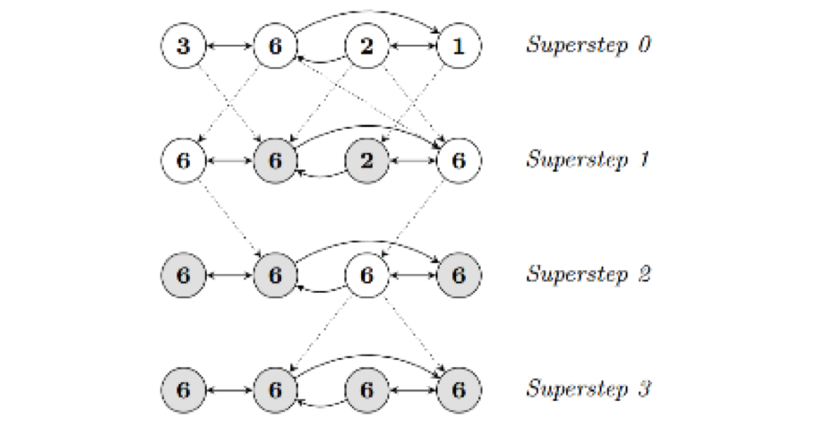
　　　　　　每个点之间在发消息的时候是独立的，即:点单纯根据方向，向以相邻点的以localId为下标的数组中插数据，互相独立，可以并行运行。Map阶段最后返回消息RDD messages: RDD[(VertexId, VD2)]

　　　　　　Map阶段的执行流程如下例所示：

　　　　　　

　　2.4.7.1.2.2 Reduce阶段

　　　　　　Reduce阶段的实现就是调用下面的代码

vertices.aggregateUsingIndex(preAgg, mergeMsg)
override def aggregateUsingIndex[VD2: ClassTag](
  messages: RDD[(VertexId, VD2)], reduceFunc: (VD2, VD2) => VD2): VertexRDD[VD2] = {
  val shuffled = messages.partitionBy(this.partitioner.get)
  val parts = partitionsRDD.zipPartitions(shuffled, true) { (thisIter, msgIter) =>
    thisIter.map(_.aggregateUsingIndex(msgIter, reduceFunc))
  }
  this.withPartitionsRDD[VD2](parts)
}

　　　　　　上面的代码通过两步实现

　　　　　　1. 对messages重新分区，分区器使用VertexRDD的partitioner。然后使用zipPartitions合并两个分区

　　　　　　2. 对等合并attr, 聚合函数使用传入的mergeMsg函数

def aggregateUsingIndex[VD2: ClassTag](
    iter: Iterator[Product2[VertexId, VD2]],
    reduceFunc: (VD2, VD2) => VD2): Self[VD2] = {
  val newMask = new BitSet(self.capacity)
  val newValues = new Array[VD2](self.capacity)
  iter.foreach { product =>
    val vid = product._1
    val vdata = product._2
    val pos = self.index.getPos(vid)
    if (pos >= 0) {
      if (newMask.get(pos)) {
        newValues(pos) = reduceFunc(newValues(pos), vdata)
      } else { // otherwise just store the new value
        newMask.set(pos)
        newValues(pos) = vdata
      }
    }
  }
  this.withValues(newValues).withMask(newMask)
}

　　　　　　根据传参，我们知道上面的代码迭代的是messagePartition，并不是每个节点都会收到消息，所以messagePartition集合最小，迭代速度会快。这段代码表示，我们根据 vetexId从index中取到其下标pos，再根据下标，从values中取到attr，存在attr就用mergeMsg合并attr，不存在就直接赋值

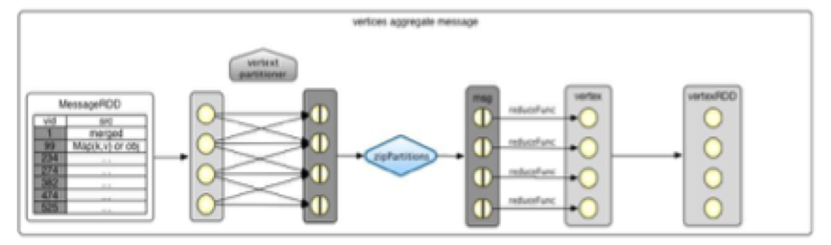
　　　　　　Reduce阶段的过程如下图所示：

　　　　　　

　　2.4.7.1.3 举例

　　　　　　下面的例子计算比用户年龄大的追随者(即followers)的平均年龄

// Import random graph generation library
import org.apache.spark.graphx.util.GraphGenerators
// Create a graph with "age" as the vertex property. Here we use a random graph for simplicity.

val graph: Graph[Double, Int] =
  GraphGenerators.logNormalGraph(sc, numVertices = 100).mapVertices( (id, _) => id.toDouble )
// Compute the number of older followers and their total age
val olderFollowers: VertexRDD[(Int, Double)] = graph.aggregateMessages[(Int, Double)](
  triplet => { // Map Function
    if (triplet.srcAttr > triplet.dstAttr) {
      // Send message to destination vertex containing counter and age
      triplet.sendToDst(1, triplet.srcAttr)
    }
  },
  // Add counter and age
  (a, b) => (a._1 + b._1, a._2 + b._2) // Reduce Function
)
// Divide total age by number of older followers to get average age of older followers
val avgAgeOfOlderFollowers: VertexRDD[Double] =
  olderFollowers.mapValues( (id, value) => value match { case (count, totalAge) => totalAge / count } )
// Display the results
avgAgeOfOlderFollowers.collect.foreach(println(_))

　　2.4.7.2 collectNeighbors

　　　　　　该方法的作用是收集每个顶点的邻居顶点的顶点和顶点属性。需要指定方向

def collectNeighbors(edgeDirection: EdgeDirection): VertexRDD[Array[(VertexId, VD)]] = {
  val nbrs = edgeDirection match {
    case EdgeDirection.Either =>
      graph.aggregateMessages[Array[(VertexId, VD)]](
        ctx => {
          ctx.sendToSrc(Array((ctx.dstId, ctx.dstAttr)))
          ctx.sendToDst(Array((ctx.srcId, ctx.srcAttr)))
        },
        (a, b) => a ++ b, TripletFields.All)
    case EdgeDirection.In => g
      raph.aggregateMessages[Array[(VertexId, VD)]](
        ctx => ctx.sendToDst(Array((ctx.srcId, ctx.srcAttr))),
        (a, b) => a ++ b, TripletFields.Src)
    case EdgeDirection.Out =>
      graph.aggregateMessages[Array[(VertexId, VD)]](
        ctx => ctx.sendToSrc(Array((ctx.dstId, ctx.dstAttr))), (a, b) => a ++ b, TripletFields.Dst)
    case EdgeDirection.Both =>
      throw new SparkException("collectEdges does not support
  EdgeDirection.Both. Use" + "EdgeDirection.Either instead.")
  }
  graph.vertices.leftJoin(nbrs) { (vid, vdata, nbrsOpt) => nbrsOpt.getOrElse(Array.empty[(VertexId, VD)])
  }
}

　　　　　　从上面的代码中，第一步是根据EdgeDirection来确定调用哪个aggregateMessages实现聚合操作。我们用满足条件EdgeDirection.Either的情况来说明。可以看到 aggregateMessages的方式消息的函数为：

ctx => {
  ctx.sendToSrc(Array((ctx.dstId, ctx.dstAttr)))
  ctx.sendToDst(Array((ctx.srcId, ctx.srcAttr)))
},

　　　　　　这个函数在处理每条边时都会同时向源顶点和目的顶点发送消息，消息内容分别为(目的顶点 id，目的顶点属性)、(源顶点 id，源顶点属性)。为什么会这样处理呢? 我们知道，每条边都由两个顶点组成，对于这个边，我需要向源顶点发送目的顶点的信息来记录它们之间的邻居关系，同理向目的顶点发送源顶点的信息来记录它们之间的邻居关系

　　　　　　Merge函数是一个集合合并操作，它合并同同一个顶点对应的所有目的顶点的信息。如下所示：

(a, b) => a ++ b

　　　　　　通过aggregateMessages获得包含邻居关系信息的VertexRDD后，把它和现有的vertices作join操作，得到每个顶点的邻居消息

　　2.4.7.3 collectNeighborlds

　　　　　　该方法的作用是收集每个顶点的邻居顶点的顶点id。它的实现和collectNeighbors非常相同。需要指定方向

def collectNeighborIds(edgeDirection: EdgeDirection): VertexRDD[Array[VertexId]] = {
  val nbrs =
    if (edgeDirection == EdgeDirection.Either) {
      graph.aggregateMessages[Array[VertexId]](
        ctx => { ctx.sendToSrc(Array(ctx.dstId));
        ctx.sendToDst(Array(ctx.srcId)) },
        _ ++ _, TripletFields.None)
    } else if (edgeDirection == EdgeDirection.Out) {
        graph.aggregateMessages[Array[VertexId]](
          ctx => ctx.sendToSrc(Array(ctx.dstId)),
          _ ++ _, TripletFields.None)
    } else if (edgeDirection == EdgeDirection.In) {
        graph.aggregateMessages[Array[VertexId]](
          ctx => ctx.sendToDst(Array(ctx.srcId)),
          _ ++ _, TripletFields.None)
    } else {
      throw new SparkException("It doesn't make sense to collect neighbor ids without a " +
  "direction. (EdgeDirection.Both is not supported; use EdgeDirection.Either instead.)")
    }
  graph.vertices.leftZipJoin(nbrs) { (vid, vdata, nbrsOpt) => nbrsOpt.getOrElse(Array.empty[VertexId])
  }
}

　　　　　　和collectNeighbors的实现不同的是，aggregateMessages函数中的sendMsg函数只发送顶点Id到源顶点和目的顶点。其它的实现基本一致

ctx => { ctx.sendToSrc(Array(ctx.dstId)); ctx.sendToDst(Array(ctx.srcId)) }

　　2.4.8 缓存操作

　　　　　　在Spark中，RDD默认是不缓存的。为了避免重复计算，当需要多次利用它们时，我们必须显示地缓存它们。GraphX中的图也有相同的方式。当利用到图多次时，确保首先访问Graph.cache()方法。

　　　　　　在迭代计算中，为了获得最佳的性能，不缓存可能是必须的。默认情况下，缓存的RDD和图会一直保留在内存中直到因为内存压力迫使它们以LRU的顺序删除。对于迭代计算，先前的迭代的中间结果将填充到缓存中。虽然它们最终会被删除，但是保存在内存中的不需要的数据将会减慢垃圾回收。只有中间结果不需要，不缓存它们是更高效的。然而，因为图是由多个RDD组成的，正确的不持久化它们是困难的。对于迭代计算，建议使用Pregel API，它可以正确的不持久化中间结果

　　　　　　GraphX中的缓存操作有cache，persist，unpersist和unpersistVertices。它们的接口分别是：

def persist(newLevel: StorageLevel = StorageLevel.MEMORY_ONLY): Graph[VD, ED]
def cache(): Graph[VD, ED]
def unpersist(blocking: Boolean = true): Graph[VD, ED]
def unpersistVertices(blocking: Boolean = true): Graph[VD, ED]

2.5 Pregel API

　　　　　　图本身是递归数据结构，顶点的属性依赖于它们邻居的属性，这些邻居的属性又依赖于自己邻居的属性。所以许多重要的图算法都是迭代的重新计算每个顶点的属性，直到满足某个确定的条件。 一系列的图并发(graph-parallel)抽象已经被提出来用来表达这些迭代算法。GraphX公开了一个类似Pregel的操作，它是广泛使用的Pregel和GraphLab抽象的一个融合

　　　　　　GraphX中实现的这个更高级的Pregel操作是一个约束到图拓扑的批量同步(bulk-synchronous)并行消息抽象。Pregel操作者执行一系列的超步(super steps)，在这些步骤中，顶点从之前的超步中接收进入(inbound)消息的总和，为顶点属性计算一个新的值，然后在以后的超步中发送消息到邻居顶点。不像Pregel而更像GraphLab，消息通过边triplet的一个函数被并行计算，消息的计算既会访问源顶点特征也会访问目的顶点特征。在超步中，没有收到消息的顶点会被跳过。当没有消息遗留时，Pregel操作停止迭代并返回最终的图

　　　　　　注意，与标准的Pregel实现不同的是，GraphX中的顶点仅仅能发送信息给邻居顶点，并且可以利用用户自定义的消息函数并行地构造消息。这些限制允许对GraphX进行额外的优化

　　　　　　下面的代码是pregel的具体实现：

def apply[VD: ClassTag, ED: ClassTag, A: ClassTag]
  (graph: Graph[VD, ED],
  initialMsg: A,
  maxIterations: Int = Int.MaxValue,
  activeDirection: EdgeDirection = EdgeDirection.Either)
  (vprog: (VertexId, VD, A) => VD,
  sendMsg: EdgeTriplet[VD, ED] => Iterator[(VertexId, A)], mergeMsg: (A, A) => A)
  : Graph[VD, ED] =
{
  var g = graph.mapVertices((vid, vdata) => vprog(vid, vdata, initialMsg)).cache()
  // 计算消息
  var messages = g.mapReduceTriplets(sendMsg, mergeMsg)
  var activeMessages = messages.count()
  // 迭代
  var prevG: Graph[VD, ED] = null
  var i = 0
  while (activeMessages > 0 && i < maxIterations) {
    // 接收消息并更新顶点
    prevG = g
    g = g.joinVertices(messages)(vprog).cache()
    val oldMessages = messages
    // 发送新消息
    messages = g.mapReduceTriplets(
      sendMsg, mergeMsg, Some((oldMessages, activeDirection))).cache()
    activeMessages = messages.count()
    i += 1
  }
  g
}

　　2.5.1 pregel计算模型

　　　　　　Pregel计算模型中有三个重要的函数，分别是vertexProgram、sendMessage和messageCombiner

　　　　　　　　vertexProgram：用户定义的顶点运行程序。它作用于每一个顶点，负责接收进来的信息，并计算新的顶点值。

　　　　　　　　sendMsg：发送消息

　　　　　　　　mergeMsg：合并消息

　　　　　　具体分析它的实现。根据代码可以知道，这个实现是一个迭代的过程。在开始迭代之前，先完成一些初始化操作：

var g= graph.mapVertices((vid,vdata) => vprog(vid,vdata, initialMsg)).cache()
// 计算消息
var messages = g.mapReduceTriplets(sendMsg, mergeMsg)
var activeMessages = messages.count()

　　　　　　程序首先用vprog函数处理图中所有的顶点，生成新的图。然后用生成的图调用聚合操作(mapReduceTriplets，实际的实现是我们前面章节讲到的aggregateMessagesWithActiveSet函数)获取聚合后的消息。activeMessages指messages这个VertexRDD中的顶点数

　　　　　　下面就开始迭代操作了。在迭代内部，分为二步:

　　　　　　1. 接收消息，并更新顶点

g = g.joinVertices(messages)(vprog).cache()
//joinVertices 的定义
def joinVertices[U: ClassTag](table: RDD[(VertexId, U)])(mapFunc: (VertexId, VD, U) => VD): Graph[VD, ED] = {
  val uf = (id: VertexId, data: VD, o: Option[U]) => {
    o match {
      case Some(u) => mapFunc(id, data, u)
      case None => data
    }
  }
  graph.outerJoinVertices(table)(uf)
}

　　　　　　这一步实际上是使用outerJoinVertices来更新顶点属性。outerJoinVertices在关联操作中有详细介绍：

　　　　　　2. 发送新消息

messages = g.mapReduceTriplets(
    sendMsg, mergeMsg, Some((oldMessages, activeDirection))).cache()

　　　　　　注意，在上面的代码中，mapReduceTriplets多了一个参数Some((oldMessages, activeDirection))。这个参数的作用是:它使我们在发送新的消息时，会忽略掉那些两端都没有接收到消息的边，减少计算量

　　2.5.2 pregel实现最短路径

import org.apache.spark.graphx._
import org.apache.spark.graphx.util.GraphGenerators
val graph: Graph[Long, Double] =
  GraphGenerators.logNormalGraph(sc, numVertices = 100).mapEdges(e => e.attr.toDouble)
val sourceId: VertexId = 42 // The ultimate source
// 初始化图
val initialGraph = graph.mapVertices((id, _) => if (id == sourceId) 0.0 else Double.PositiveInfinity)
val sssp = initialGraph.pregel(Double.PositiveInfinity)(
  (id, dist, newDist) => math.min(dist, newDist), // Vertex Program
  triplet => { // Send Message
    if (triplet.srcAttr + triplet.attr < triplet.dstAttr) {
      Iterator((triplet.dstId, triplet.srcAttr + triplet.attr))
    } else {
      Iterator.empty
    }
  },
  (a,b) => math.min(a,b) // Merge Message
)
println(sssp.vertices.collect.mkString("\n"))

　　　　　　上面的例子中，Vertex Program函数定义如下:

(id, dist, newDist) => math.min(dist, newDist)

　　　　　　这个函数的定义显而易见，当两个消息来的时候，取它们当中路径的最小值。同理Merge Message函数也是同样的含义Send Message函数中，会首先比较triplet.srcAttr + triplet.attr 和triplet.dstAttr，即比较加上边的属性后，这个值是否小于目的节点的属性，如果小于，则发送消息到目的顶点