python金融反欺诈-项目实战
python风控建模实战lendingClub(博主录制,catboost,lightgbm建模,2K超清分辨率)
https://study.163.com/course/courseMain.htm?courseId=1005988013&share=2&shareId=400000000398149

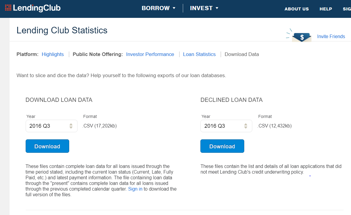
## 1. Data Lending Club 2016年Q3数据:https://www.lendingclub.com/info/download-data.action
参考:http://kldavenport.com/lending-club-data-analysis-revisted-with-python/
import pandas as pd

import numpy as np

import matplotlib.pyplot as plt

import seaborn as sns

%matplotlib inline
df = pd.read_csv("./LoanStats_2016Q3.csv",skiprows=1,low_memory=False)df.info()df.head(3)| id | member_id | loan_amnt | funded_amnt | funded_amnt_inv | term | int_rate | installment | grade | sub_grade | … | sec_app_earliest_cr_line | sec_app_inq_last_6mths | sec_app_mort_acc | sec_app_open_acc | sec_app_revol_util | sec_app_open_il_6m | sec_app_num_rev_accts | sec_app_chargeoff_within_12_mths | sec_app_collections_12_mths_ex_med | sec_app_mths_since_last_major_derog | |
|---|---|---|---|---|---|---|---|---|---|---|---|---|---|---|---|---|---|---|---|---|---|
| 0 | NaN | NaN | 15000.0 | 15000.0 | 15000.0 | 36 months | 13.99% | 512.60 | C | C3 | … | NaN | NaN | NaN | NaN | NaN | NaN | NaN | NaN | NaN | NaN |
| 1 | NaN | NaN | 2600.0 | 2600.0 | 2600.0 | 36 months | 8.99% | 82.67 | B | B1 | … | NaN | NaN | NaN | NaN | NaN | NaN | NaN | NaN | NaN | NaN |
| 2 | NaN | NaN | 32200.0 | 32200.0 | 32200.0 | 60 months | 21.49% | 880.02 | D | D5 | … | NaN | NaN | NaN | NaN | NaN | NaN | NaN | NaN | NaN | NaN |
3 rows × 122 columns
## 2. Keep what we need
# .ix[row slice, column slice]

df.ix[:4,:7]| id | member_id | loan_amnt | funded_amnt | funded_amnt_inv | term | int_rate | |
|---|---|---|---|---|---|---|---|
| 0 | NaN | NaN | 15000.0 | 15000.0 | 15000.0 | 36 months | 13.99% |
| 1 | NaN | NaN | 2600.0 | 2600.0 | 2600.0 | 36 months | 8.99% |
| 2 | NaN | NaN | 32200.0 | 32200.0 | 32200.0 | 60 months | 21.49% |
| 3 | NaN | NaN | 10000.0 | 10000.0 | 10000.0 | 36 months | 11.49% |
| 4 | NaN | NaN | 6000.0 | 6000.0 | 6000.0 | 36 months | 13.49% |
df.drop('id',1,inplace=True)

df.drop('member_id',1,inplace=True)
df.int_rate = pd.Series(df.int_rate).str.replace('%', '').astype(float)df.ix[:4,:7]| loan_amnt | funded_amnt | funded_amnt_inv | term | int_rate | installment | grade | |
|---|---|---|---|---|---|---|---|
| 0 | 15000.0 | 15000.0 | 15000.0 | 36 months | 13.99 | 512.60 | C |
| 1 | 2600.0 | 2600.0 | 2600.0 | 36 months | 8.99 | 82.67 | B |
| 2 | 32200.0 | 32200.0 | 32200.0 | 60 months | 21.49 | 880.02 | D |
| 3 | 10000.0 | 10000.0 | 10000.0 | 36 months | 11.49 | 329.72 | B |
| 4 | 6000.0 | 6000.0 | 6000.0 | 36 months | 13.49 | 203.59 | C |
### Loan Amount Requested Verus the Funded Amount
print (df.loan_amnt != df.funded_amnt).value_counts()False 99120 True 4 dtype: int64
df.query('loan_amnt != funded_amnt').head(5)| loan_amnt | funded_amnt | funded_amnt_inv | term | int_rate | installment | grade | sub_grade | emp_title | emp_length | … | sec_app_earliest_cr_line | sec_app_inq_last_6mths | sec_app_mort_acc | sec_app_open_acc | sec_app_revol_util | sec_app_open_il_6m | sec_app_num_rev_accts | sec_app_chargeoff_within_12_mths | sec_app_collections_12_mths_ex_med | sec_app_mths_since_last_major_derog | |
|---|---|---|---|---|---|---|---|---|---|---|---|---|---|---|---|---|---|---|---|---|---|
| 99120 | NaN | NaN | NaN | NaN | NaN | NaN | NaN | NaN | NaN | NaN | … | NaN | NaN | NaN | NaN | NaN | NaN | NaN | NaN | NaN | NaN |
| 99121 | NaN | NaN | NaN | NaN | NaN | NaN | NaN | NaN | NaN | NaN | … | NaN | NaN | NaN | NaN | NaN | NaN | NaN | NaN | NaN | NaN |
| 99122 | NaN | NaN | NaN | NaN | NaN | NaN | NaN | NaN | NaN | NaN | … | NaN | NaN | NaN | NaN | NaN | NaN | NaN | NaN | NaN | NaN |
| 99123 | NaN | NaN | NaN | NaN | NaN | NaN | NaN | NaN | NaN | NaN | … | NaN | NaN | NaN | NaN | NaN | NaN | NaN | NaN | NaN | NaN |
4 rows × 120 columns
df.dropna(axis=0, how='all',inplace=True)df.info()df.dropna(axis=1, how='all',inplace=True)df.info()df.ix[:5,8:15]| emp_title | emp_length | home_ownership | annual_inc | verification_status | issue_d | loan_status | |
|---|---|---|---|---|---|---|---|
| 0 | Fiscal Director | 2 years | RENT | 55000.0 | Not Verified | Sep-16 | Current |
| 1 | Loaner Coordinator | 3 years | RENT | 35000.0 | Source Verified | Sep-16 | Fully Paid |
| 2 | warehouse/supervisor | 10+ years | MORTGAGE | 65000.0 | Not Verified | Sep-16 | Fully Paid |
| 3 | Teacher | 10+ years | OWN | 55900.0 | Not Verified | Sep-16 | Current |
| 4 | SERVICE MGR | 5 years | RENT | 33000.0 | Not Verified | Sep-16 | Current |
| 5 | General Manager | 10+ years | MORTGAGE | 109000.0 | Source Verified | Sep-16 | Current |
### emp_title: employment title
print df.emp_title.value_counts().head()

print df.emp_title.value_counts().tail()

df.emp_title.unique().shape
Teacher 1931 Manager 1701 Owner 990 Supervisor 785 Driver 756 Name: emp_title, dtype: int64 Agent Services Representative 1 Operator Bridge Tunnel 1 Reg Medical Assistant/Referral Spec. 1 Home Health Care 1 rounds cook 1 Name: emp_title, dtype: int64 (37421,)
df.drop(['emp_title'],1, inplace=True)df.ix[:5,8:15]| emp_length | home_ownership | annual_inc | verification_status | issue_d | loan_status | pymnt_plan | |
|---|---|---|---|---|---|---|---|
| 0 | 2 years | RENT | 55000.0 | Not Verified | Sep-16 | Current | n |
| 1 | 3 years | RENT | 35000.0 | Source Verified | Sep-16 | Fully Paid | n |
| 2 | 10+ years | MORTGAGE | 65000.0 | Not Verified | Sep-16 | Fully Paid | n |
| 3 | 10+ years | OWN | 55900.0 | Not Verified | Sep-16 | Current | n |
| 4 | 5 years | RENT | 33000.0 | Not Verified | Sep-16 | Current | n |
| 5 | 10+ years | MORTGAGE | 109000.0 | Source Verified | Sep-16 | Current | n |
### emp_length: employment length
df.emp_length.value_counts()10+ years 34219 2 years 9066 3 years 7925
df.replace('n/a', np.nan,inplace=True)

df.emp_length.fillna(value=0,inplace=True)

df['emp_length'].replace(to_replace='[^0-9]+', value='', inplace=True, regex=True)

df['emp_length'] = df['emp_length'].astype(int)df.emp_length.value_counts()10 34219 1 14095 2 9066 3 7925 5 6170 4 6022 0 5922 6 4406 8 4168 9 3922 7 3205 Name: emp_length, dtype: int64 ### verification status:”Indicates if income was verified by LC, not verified, or if the income source was verified”
df.verification_status.value_counts()Source Verified 40781 Verified 31356 Not Verified 26983 Name: verification_status, dtype: int64 ### Target: Loan Statuses
df.info()df.columnsIndex([u’loan_amnt’, u’funded_amnt’, u’funded_amnt_inv’, u’term’, u’int_rate’, u’installment’, u’grade’, u’sub_grade’, u’emp_length’, u’home_ownership’, … u’num_tl_90g_dpd_24m’, u’num_tl_op_past_12m’, u’pct_tl_nvr_dlq’, u’percent_bc_gt_75’, u’pub_rec_bankruptcies’, u’tax_liens’, u’tot_hi_cred_lim’, u’total_bal_ex_mort’, u’total_bc_limit’, u’total_il_high_credit_limit’], dtype=’object’, length=107)
pd.unique(df['loan_status'].values.ravel())array([‘Current’, ‘Fully Paid’, ‘Late (31-120 days)’, ‘Charged Off’, ‘Late (16-30 days)’, ‘In Grace Period’, ‘Default’], dtype=object)
for col in df.select_dtypes(include=['object']).columns:

    print ("Column {} has {} unique instances".format( col, len(df[col].unique())) )
Column term has 2 unique instances Column grade has 7 unique instances Column sub_grade has 35 unique instances Column home_ownership has 4 unique instances Column verification_status has 3 unique instances Column issue_d has 3 unique instances Column loan_status has 7 unique instances Column pymnt_plan has 2 unique instances Column desc has 6 unique instances Column purpose has 13 unique instances Column title has 13 unique instances Column zip_code has 873 unique instances Column addr_state has 50 unique instances Column earliest_cr_line has 614 unique instances Column revol_util has 1087 unique instances Column initial_list_status has 2 unique instances Column last_pymnt_d has 13 unique instances Column next_pymnt_d has 4 unique instances Column last_credit_pull_d has 14 unique instances Column application_type has 3 unique instances Column verification_status_joint has 2 unique instances
# 处理对象类型的缺失,unique

df.select_dtypes(include=['O']).describe().T.\

assign(missing_pct=df.apply(lambda x : (len(x)-x.count())/float(len(x))))| count | unique | top | freq | missing_pct | |
|---|---|---|---|---|---|
| term | 99120 | 2 | 36 months | 73898 | 0.000000 |
| grade | 99120 | 7 | C | 32846 | 0.000000 |
| sub_grade | 99120 | 35 | B5 | 8322 | 0.000000 |
| home_ownership | 99120 | 4 | MORTGAGE | 46761 | 0.000000 |
| verification_status | 99120 | 3 | Source Verified | 40781 | 0.000000 |
| issue_d | 99120 | 3 | Aug-16 | 36280 | 0.000000 |
| loan_status | 99120 | 7 | Current | 79445 | 0.000000 |
| pymnt_plan | 99120 | 2 | n | 99074 | 0.000000 |
| desc | 6 | 5 | 2 | 0.999939 | |
| purpose | 99120 | 13 | debt_consolidation | 57682 | 0.000000 |
| title | 93693 | 12 | Debt consolidation | 53999 | 0.054752 |
| zip_code | 99120 | 873 | 112xx | 1125 | 0.000000 |
| addr_state | 99120 | 50 | CA | 13352 | 0.000000 |
| earliest_cr_line | 99120 | 614 | Aug-03 | 796 | 0.000000 |
| revol_util | 99060 | 1086 | 0% | 440 | 0.000605 |
| initial_list_status | 99120 | 2 | w | 71869 | 0.000000 |
| last_pymnt_d | 98991 | 12 | Jun-17 | 81082 | 0.001301 |
| next_pymnt_d | 83552 | 3 | Jul-17 | 83527 | 0.157062 |
| last_credit_pull_d | 99115 | 13 | Jun-17 | 89280 | 0.000050 |
| application_type | 99120 | 3 | INDIVIDUAL | 98565 | 0.000000 |
| verification_status_joint | 517 | 1 | Not Verified | 517 | 0.994784 |
df.revol_util = pd.Series(df.revol_util).str.replace('%', '').astype(float)# missing_pct
df.drop('desc',1,inplace=True)
df.drop('verification_status_joint',1,inplace=True)df.drop('zip_code',1,inplace=True)
df.drop('addr_state',1,inplace=True)
df.drop('earliest_cr_line',1,inplace=True)
df.drop('revol_util',1,inplace=True)
df.drop('purpose',1,inplace=True)
df.drop('title',1,inplace=True)
df.drop('term',1,inplace=True)
df.drop('issue_d',1,inplace=True)
# df.drop('',1,inplace=True)
# 贷后相关的字段
df.drop(['out_prncp','out_prncp_inv','total_pymnt',
'total_pymnt_inv','total_rec_prncp', 'grade', 'sub_grade'] ,1, inplace=True)
df.drop(['total_rec_int','total_rec_late_fee',
'recoveries','collection_recovery_fee',
'collection_recovery_fee' ],1, inplace=True)
df.drop(['last_pymnt_d','last_pymnt_amnt',
'next_pymnt_d','last_credit_pull_d'],1, inplace=True)
df.drop(['policy_code'],1, inplace=True)df.info()df.ix[:5,:10]| loan_amnt | funded_amnt | funded_amnt_inv | int_rate | installment | emp_length | home_ownership | annual_inc | verification_status | loan_status | |
|---|---|---|---|---|---|---|---|---|---|---|
| 0 | 15000.0 | 15000.0 | 15000.0 | 13.99 | 512.60 | 2 | RENT | 55000.0 | Not Verified | Current |
| 1 | 2600.0 | 2600.0 | 2600.0 | 8.99 | 82.67 | 3 | RENT | 35000.0 | Source Verified | Fully Paid |
| 2 | 32200.0 | 32200.0 | 32200.0 | 21.49 | 880.02 | 10 | MORTGAGE | 65000.0 | Not Verified | Fully Paid |
| 3 | 10000.0 | 10000.0 | 10000.0 | 11.49 | 329.72 | 10 | OWN | 55900.0 | Not Verified | Current |
| 4 | 6000.0 | 6000.0 | 6000.0 | 13.49 | 203.59 | 5 | RENT | 33000.0 | Not Verified | Current |
| 5 | 30000.0 | 30000.0 | 30000.0 | 13.99 | 697.90 | 10 | MORTGAGE | 109000.0 | Source Verified | Current |
df.ix[:5,10:21]| pymnt_plan | dti | delinq_2yrs | inq_last_6mths | mths_since_last_delinq | mths_since_last_record | open_acc | pub_rec | revol_bal | total_acc | initial_list_status | |
|---|---|---|---|---|---|---|---|---|---|---|---|
| 0 | n | 23.78 | 1.0 | 0.0 | 7.0 | NaN | 22.0 | 0.0 | 21345.0 | 43.0 | f |
| 1 | n | 6.73 | 0.0 | 0.0 | NaN | NaN | 14.0 | 0.0 | 720.0 | 24.0 | w |
| 2 | n | 11.71 | 0.0 | 1.0 | NaN | 87.0 | 17.0 | 1.0 | 11987.0 | 34.0 | w |
| 3 | n | 26.21 | 0.0 | 2.0 | NaN | NaN | 15.0 | 0.0 | 17209.0 | 62.0 | w |
| 4 | n | 19.05 | 0.0 | 0.0 | NaN | NaN | 3.0 | 0.0 | 4576.0 | 11.0 | f |
| 5 | n | 16.24 | 0.0 | 0.0 | NaN | NaN | 17.0 | 0.0 | 11337.0 | 39.0 | w |
print df.columns

print df.head(1).values

df.info()
Index([u’loan_amnt’, u’funded_amnt’, u’funded_amnt_inv’, u’int_rate’, u’installment’, u’emp_length’, u’home_ownership’, u’annual_inc’, u’verification_status’, u’loan_status’, u’pymnt_plan’, u’dti’, u’delinq_2yrs’, u’inq_last_6mths’, u’mths_since_last_delinq’, u’mths_since_last_record’, u’open_acc’, u’pub_rec’, u’revol_bal’, u’total_acc’, u’initial_list_status’, u’collections_12_mths_ex_med’, u’mths_since_last_major_derog’, u’application_type’, u’annual_inc_joint’, u’dti_joint’, u’acc_now_delinq’, u’tot_coll_amt’, u’tot_cur_bal’, u’open_acc_6m’, u’open_il_6m’, u’open_il_12m’, u’open_il_24m’, u’mths_since_rcnt_il’, u’total_bal_il’, u’il_util’, u’open_rv_12m’, u’open_rv_24m’, u’max_bal_bc’, u’all_util’, u’total_rev_hi_lim’, u’inq_fi’, u’total_cu_tl’, u’inq_last_12m’, u’acc_open_past_24mths’, u’avg_cur_bal’, u’bc_open_to_buy’, u’bc_util’, u’chargeoff_within_12_mths’, u’delinq_amnt’, u’mo_sin_old_il_acct’, u’mo_sin_old_rev_tl_op’, u’mo_sin_rcnt_rev_tl_op’, u’mo_sin_rcnt_tl’, u’mort_acc’, u’mths_since_recent_bc’, u’mths_since_recent_bc_dlq’, u’mths_since_recent_inq’, u’mths_since_recent_revol_delinq’, u’num_accts_ever_120_pd’, u’num_actv_bc_tl’, u’num_actv_rev_tl’, u’num_bc_sats’, u’num_bc_tl’, u’num_il_tl’, u’num_op_rev_tl’, u’num_rev_accts’, u’num_rev_tl_bal_gt_0’, u’num_sats’, u’num_tl_120dpd_2m’, u’num_tl_30dpd’, u’num_tl_90g_dpd_24m’, u’num_tl_op_past_12m’, u’pct_tl_nvr_dlq’, u’percent_bc_gt_75’, u’pub_rec_bankruptcies’, u’tax_liens’, u’tot_hi_cred_lim’, u’total_bal_ex_mort’, u’total_bc_limit’, u’total_il_high_credit_limit’], dtype=’object’) [[15000.0 15000.0 15000.0 13.99 512.6 2 ‘RENT’ 55000.0 ‘Not Verified’ ‘Current’ ‘n’ 23.78 1.0 0.0 7.0 nan 22.0 0.0 21345.0 43.0 ‘f’ 0.0 nan ‘INDIVIDUAL’ nan nan 0.0 0.0 140492.0 3.0 10.0 2.0 3.0 11.0 119147.0 101.0 3.0 4.0 14612.0 83.0 39000.0 1.0 6.0 0.0 7.0 6386.0 9645.0 73.1 0.0 0.0 157.0 248.0 4.0 4.0 0.0 4.0 7.0 22.0 7.0 0.0 5.0 9.0 6.0 7.0 25.0 11.0 18.0 9.0 22.0 0.0 0.0 0.0 5.0 100.0 33.3 0.0 0.0 147587.0 140492.0 30200.0 108587.0]]
df.select_dtypes(include=['float']).describe().T.\

assign(missing_pct=df.apply(lambda x : (len(x)-x.count())/float(len(x))))
/Users/ting/anaconda/lib/python2.7/site-packages/numpy/lib/function_base.py:3834: RuntimeWarning: Invalid value encountered in percentile RuntimeWarning)
| count | mean | std | min | 25% | 50% | 75% | max | missing_pct | |
|---|---|---|---|---|---|---|---|---|---|
| loan_amnt | 99120.0 | 14170.570521 | 8886.138758 | 1000.00 | 7200.00 | 12000.00 | 20000.00 | 40000.00 | 0.000000 |
| funded_amnt | 99120.0 | 14170.570521 | 8886.138758 | 1000.00 | 7200.00 | 12000.00 | 20000.00 | 40000.00 | 0.000000 |
| funded_amnt_inv | 99120.0 | 14166.087823 | 8883.301328 | 1000.00 | 7200.00 | 12000.00 | 20000.00 | 40000.00 | 0.000000 |
| int_rate | 99120.0 | 13.723641 | 4.873910 | 5.32 | 10.49 | 12.79 | 15.59 | 30.99 | 0.000000 |
| installment | 99120.0 | 432.718654 | 272.678596 | 30.12 | 235.24 | 361.38 | 569.83 | 1535.71 | 0.000000 |
| annual_inc | 99120.0 | 78488.850081 | 72694.186060 | 0.00 | 48000.00 | 65448.00 | 94000.00 | 8400000.00 | 0.000000 |
| dti | 99120.0 | 18.348651 | 64.057603 | 0.00 | 11.91 | 17.60 | 23.90 | 9999.00 | 0.000000 |
| delinq_2yrs | 99120.0 | 0.381901 | 0.988996 | 0.00 | 0.00 | 0.00 | 0.00 | 21.00 | 0.000000 |
| inq_last_6mths | 99120.0 | 0.570521 | 0.863796 | 0.00 | 0.00 | 0.00 | 1.00 | 5.00 | 0.000000 |
| mths_since_last_delinq | 53366.0 | 33.229172 | 21.820407 | 0.00 | NaN | NaN | NaN | 142.00 | 0.461602 |
| mths_since_last_record | 19792.0 | 67.267886 | 24.379343 | 0.00 | NaN | NaN | NaN | 119.00 | 0.800323 |
| open_acc | 99120.0 | 11.718251 | 5.730585 | 1.00 | 8.00 | 11.00 | 15.00 | 86.00 | 0.000000 |
| pub_rec | 99120.0 | 0.266596 | 0.719193 | 0.00 | 0.00 | 0.00 | 0.00 | 61.00 | 0.000000 |
| revol_bal | 99120.0 | 15536.628047 | 21537.790599 | 0.00 | 5657.00 | 10494.00 | 18501.50 | 876178.00 | 0.000000 |
| total_acc | 99120.0 | 24.033545 | 11.929761 | 2.00 | 15.00 | 22.00 | 31.00 | 119.00 | 0.000000 |
| collections_12_mths_ex_med | 99120.0 | 0.021640 | 0.168331 | 0.00 | 0.00 | 0.00 | 0.00 | 10.00 | 0.000000 |
| mths_since_last_major_derog | 29372.0 | 44.449612 | 22.254529 | 0.00 | NaN | NaN | NaN | 165.00 | 0.703672 |
| annual_inc_joint | 517.0 | 118120.418472 | 51131.323819 | 26943.12 | NaN | NaN | NaN | 400000.00 | 0.994784 |
| dti_joint | 517.0 | 18.637621 | 6.602016 | 2.56 | NaN | NaN | NaN | 48.58 | 0.994784 |
| acc_now_delinq | 99120.0 | 0.006709 | 0.086902 | 0.00 | 0.00 | 0.00 | 0.00 | 4.00 | 0.000000 |
| tot_coll_amt | 99120.0 | 281.797639 | 1840.699443 | 0.00 | 0.00 | 0.00 | 0.00 | 172575.00 | 0.000000 |
| tot_cur_bal | 99120.0 | 138845.606144 | 156736.843591 | 0.00 | 28689.00 | 76447.50 | 207194.75 | 3764968.00 | 0.000000 |
| open_acc_6m | 99120.0 | 0.978743 | 1.176973 | 0.00 | 0.00 | 1.00 | 2.00 | 13.00 | 0.000000 |
| open_il_6m | 99120.0 | 2.825888 | 3.109225 | 0.00 | 1.00 | 2.00 | 3.00 | 43.00 | 0.000000 |
| open_il_12m | 99120.0 | 0.723467 | 0.973888 | 0.00 | 0.00 | 0.00 | 1.00 | 13.00 | 0.000000 |
| open_il_24m | 99120.0 | 1.624818 | 1.656628 | 0.00 | 0.00 | 1.00 | 2.00 | 26.00 | 0.000000 |
| mths_since_rcnt_il | 96469.0 | 21.362531 | 26.563455 | 0.00 | NaN | NaN | NaN | 503.00 | 0.026745 |
| total_bal_il | 99120.0 | 35045.324193 | 41981.617996 | 0.00 | 9179.00 | 23199.00 | 45672.00 | 1547285.00 | 0.000000 |
| il_util | 85480.0 | 71.599158 | 23.306731 | 0.00 | NaN | NaN | NaN | 1000.00 | 0.137611 |
| open_rv_12m | 99120.0 | 1.408142 | 1.570068 | 0.00 | 0.00 | 1.00 | 2.00 | 24.00 | 0.000000 |
| … | … | … | … | … | … | … | … | … | … |
| mo_sin_old_rev_tl_op | 99120.0 | 177.634322 | 95.327498 | 3.00 | 115.00 | 160.00 | 227.00 | 901.00 | 0.000000 |
| mo_sin_rcnt_rev_tl_op | 99120.0 | 13.145369 | 16.695022 | 0.00 | 3.00 | 8.00 | 16.00 | 274.00 | 0.000000 |
| mo_sin_rcnt_tl | 99120.0 | 7.833232 | 8.649843 | 0.00 | 3.00 | 5.00 | 10.00 | 268.00 | 0.000000 |
| mort_acc | 99120.0 | 1.467585 | 1.799513 | 0.00 | 0.00 | 1.00 | 2.00 | 45.00 | 0.000000 |
| mths_since_recent_bc | 98067.0 | 23.623512 | 31.750632 | 0.00 | NaN | NaN | NaN | 546.00 | 0.010623 |
| mths_since_recent_bc_dlq | 26018.0 | 38.095280 | 22.798229 | 0.00 | NaN | NaN | NaN | 162.00 | 0.737510 |
| mths_since_recent_inq | 89254.0 | 6.626504 | 5.967648 | 0.00 | NaN | NaN | NaN | 25.00 | 0.099536 |
| mths_since_recent_revol_delinq | 36606.0 | 34.393132 | 22.371813 | 0.00 | NaN | NaN | NaN | 165.00 | 0.630690 |
| num_accts_ever_120_pd | 99120.0 | 0.594703 | 1.508027 | 0.00 | 0.00 | 0.00 | 1.00 | 36.00 | 0.000000 |
| num_actv_bc_tl | 99120.0 | 3.628218 | 2.302668 | 0.00 | 2.00 | 3.00 | 5.00 | 47.00 | 0.000000 |
| num_actv_rev_tl | 99120.0 | 5.625272 | 3.400185 | 0.00 | 3.00 | 5.00 | 7.00 | 59.00 | 0.000000 |
| num_bc_sats | 99120.0 | 4.645581 | 3.013399 | 0.00 | 3.00 | 4.00 | 6.00 | 61.00 | 0.000000 |
| num_bc_tl | 99120.0 | 7.416041 | 4.546112 | 0.00 | 4.00 | 7.00 | 10.00 | 67.00 | 0.000000 |
| num_il_tl | 99120.0 | 8.597437 | 7.528533 | 0.00 | 4.00 | 7.00 | 11.00 | 107.00 | 0.000000 |
| num_op_rev_tl | 99120.0 | 8.198820 | 4.710348 | 0.00 | 5.00 | 7.00 | 10.00 | 79.00 | 0.000000 |
| num_rev_accts | 99120.0 | 13.726312 | 7.963791 | 2.00 | 8.00 | 12.00 | 18.00 | 104.00 | 0.000000 |
| num_rev_tl_bal_gt_0 | 99120.0 | 5.566293 | 3.286135 | 0.00 | 3.00 | 5.00 | 7.00 | 59.00 | 0.000000 |
| num_sats | 99120.0 | 11.673497 | 5.709513 | 1.00 | 8.00 | 11.00 | 14.00 | 85.00 | 0.000000 |
| num_tl_120dpd_2m | 95661.0 | 0.001108 | 0.035695 | 0.00 | NaN | NaN | NaN | 4.00 | 0.034897 |
| num_tl_30dpd | 99120.0 | 0.004348 | 0.068650 | 0.00 | 0.00 | 0.00 | 0.00 | 3.00 | 0.000000 |
| num_tl_90g_dpd_24m | 99120.0 | 0.101332 | 0.567112 | 0.00 | 0.00 | 0.00 | 0.00 | 20.00 | 0.000000 |
| num_tl_op_past_12m | 99120.0 | 2.254752 | 1.960084 | 0.00 | 1.00 | 2.00 | 3.00 | 24.00 | 0.000000 |
| pct_tl_nvr_dlq | 99120.0 | 93.262828 | 9.696646 | 0.00 | 90.00 | 96.90 | 100.00 | 100.00 | 0.000000 |
| percent_bc_gt_75 | 98006.0 | 42.681332 | 36.296425 | 0.00 | NaN | NaN | NaN | 100.00 | 0.011239 |
| pub_rec_bankruptcies | 99120.0 | 0.150262 | 0.407706 | 0.00 | 0.00 | 0.00 | 0.00 | 8.00 | 0.000000 |
| tax_liens | 99120.0 | 0.075393 | 0.517275 | 0.00 | 0.00 | 0.00 | 0.00 | 61.00 | 0.000000 |
| tot_hi_cred_lim | 99120.0 | 172185.283394 | 175273.669652 | 2500.00 | 49130.75 | 108020.50 | 248473.25 | 3953111.00 | 0.000000 |
| total_bal_ex_mort | 99120.0 | 50818.694078 | 48976.640478 | 0.00 | 20913.00 | 37747.50 | 64216.25 | 1548128.00 | 0.000000 |
| total_bc_limit | 99120.0 | 20862.228420 | 20721.900664 | 0.00 | 7700.00 | 14700.00 | 27000.00 | 520500.00 | 0.000000 |
| total_il_high_credit_limit | 99120.0 | 44066.340375 | 44473.458730 | 0.00 | 15750.00 | 33183.00 | 58963.25 | 2000000.00 | 0.000000 |
74 rows × 9 columns
df.drop('annual_inc_joint',1,inplace=True)

df.drop('dti_joint',1,inplace=True)
df.select_dtypes(include=['int']).describe().T.\
assign(missing_pct=df.apply(lambda x : (len(x)-x.count())/float(len(x))))| count | mean | std | min | 25% | 50% | 75% | max | missing_pct | |
|---|---|---|---|---|---|---|---|---|---|
| emp_length | 99120.0 | 5.757092 | 3.770359 | 0.0 | 2.0 | 6.0 | 10.0 | 10.0 | 0.0 |
Target: Loan Statuses
df['loan_status'].value_counts()

# .plot(kind='bar')
79445
Fully Paid 13066
Charged Off 2502
Late (31-120 days) 2245
In Grace Period 1407
Late (16-30 days) 454
Default 1
Name: loan_status, dtype: int64df.loan_status.replace('Fully Paid', int(1),inplace=True)
df.loan_status.replace('Current', int(1),inplace=True)
df.loan_status.replace('Late (16-30 days)', int(0),inplace=True)
df.loan_status.replace('Late (31-120 days)', int(0),inplace=True)
df.loan_status.replace('Charged Off', np.nan,inplace=True)
df.loan_status.replace('In Grace Period', np.nan,inplace=True)
df.loan_status.replace('Default', np.nan,inplace=True)
# df.loan_status.astype('int')
df.loan_status.value_counts()1.0 92511
0.0 2699
Name: loan_status, dtype: int64
# df.loan_status

df.dropna(subset=['loan_status'],inplace=True)
Highly Correlated Data
cor = df.corr()

cor.loc[:,:] = np.tril(cor, k=-1) # below main lower triangle of an array

cor = cor.stack()

cor[(cor > 0.55) | (cor < -0.55)]
funded_amnt loan_amnt 1.000000
funded_amnt_inv loan_amnt 0.999994
funded_amnt 0.999994
installment loan_amnt 0.953380
funded_amnt 0.953380
funded_amnt_inv 0.953293
mths_since_last_delinq delinq_2yrs -0.551275
total_acc open_acc 0.722950
mths_since_last_major_derog mths_since_last_delinq 0.685642
open_il_24m open_il_12m 0.760219
total_bal_il open_il_6m 0.566551
open_rv_12m open_acc_6m 0.623975
open_rv_24m open_rv_12m 0.774954
max_bal_bc revol_bal 0.551409
all_util il_util 0.594925
total_rev_hi_lim revol_bal 0.815351
inq_last_12m inq_fi 0.563011
acc_open_past_24mths open_acc_6m 0.553181
open_il_24m 0.570853
open_rv_12m 0.657606
open_rv_24m 0.848964
avg_cur_bal tot_cur_bal 0.828457
bc_open_to_buy total_rev_hi_lim 0.626380
bc_util all_util 0.569469
mo_sin_rcnt_tl mo_sin_rcnt_rev_tl_op 0.606065
mort_acc tot_cur_bal 0.551198
mths_since_recent_bc mo_sin_rcnt_rev_tl_op 0.614262
mths_since_recent_bc_dlq mths_since_last_delinq 0.751613
mths_since_last_major_derog 0.553022
mths_since_recent_revol_delinq mths_since_last_delinq 0.853573
...
num_sats total_acc 0.720022
num_actv_bc_tl 0.552957
num_actv_rev_tl 0.665429
num_bc_sats 0.630778
num_op_rev_tl 0.826946
num_rev_accts 0.663595
num_rev_tl_bal_gt_0 0.668573
num_tl_30dpd acc_now_delinq 0.801444
num_tl_90g_dpd_24m delinq_2yrs 0.669267
num_tl_op_past_12m open_acc_6m 0.722131
open_il_12m 0.557902
open_rv_12m 0.844841
open_rv_24m 0.660265
acc_open_past_24mths 0.774867
pct_tl_nvr_dlq num_accts_ever_120_pd -0.592502
percent_bc_gt_75 bc_util 0.844108
pub_rec_bankruptcies pub_rec 0.580798
tax_liens pub_rec 0.752084
tot_hi_cred_lim tot_cur_bal 0.982693
avg_cur_bal 0.795652
mort_acc 0.560840
total_bal_ex_mort total_bal_il 0.902486
total_bc_limit max_bal_bc 0.581536
total_rev_hi_lim 0.775151
bc_open_to_buy 0.834159
num_bc_sats 0.633461
total_il_high_credit_limit open_il_6m 0.552023
total_bal_il 0.960349
num_il_tl 0.583329
total_bal_ex_mort 0.889238
dtype: float64
df.drop(['funded_amnt','funded_amnt_inv', 'installment'], axis=1, inplace=True)2. Our Model
from sklearn.model_selection import train_test_split

from sklearn.model_selection import GridSearchCV

from sklearn import ensemble

from sklearn.preprocessing import OneHotEncoder #https://ljalphabeta.gitbooks.io/python-/content/categorical_data.html
Y = df.loan_status
X = df.drop('loan_status',1,inplace=False)print Y.shape
print sum(Y)(95210,)
92511.0X = pd.get_dummies(X)print X.columns
print X.head(1).values
X.info()Index([u'loan_amnt', u'int_rate', u'emp_length', u'annual_inc', u'dti',
u'delinq_2yrs', u'inq_last_6mths', u'mths_since_last_delinq',
u'mths_since_last_record', u'open_acc', u'pub_rec', u'revol_bal',
u'total_acc', u'collections_12_mths_ex_med',
u'mths_since_last_major_derog', u'acc_now_delinq', u'tot_coll_amt',
u'tot_cur_bal', u'open_acc_6m', u'open_il_6m', u'open_il_12m',
u'open_il_24m', u'mths_since_rcnt_il', u'total_bal_il', u'il_util',
u'open_rv_12m', u'open_rv_24m', u'max_bal_bc', u'all_util',
u'total_rev_hi_lim', u'inq_fi', u'total_cu_tl', u'inq_last_12m',
u'acc_open_past_24mths', u'avg_cur_bal', u'bc_open_to_buy', u'bc_util',
u'chargeoff_within_12_mths', u'delinq_amnt', u'mo_sin_old_il_acct',
u'mo_sin_old_rev_tl_op', u'mo_sin_rcnt_rev_tl_op', u'mo_sin_rcnt_tl',
u'mort_acc', u'mths_since_recent_bc', u'mths_since_recent_bc_dlq',
u'mths_since_recent_inq', u'mths_since_recent_revol_delinq',
u'num_accts_ever_120_pd', u'num_actv_bc_tl', u'num_actv_rev_tl',
u'num_bc_sats', u'num_bc_tl', u'num_il_tl', u'num_op_rev_tl',
u'num_rev_accts', u'num_rev_tl_bal_gt_0', u'num_sats',
u'num_tl_120dpd_2m', u'num_tl_30dpd', u'num_tl_90g_dpd_24m',
u'num_tl_op_past_12m', u'pct_tl_nvr_dlq', u'percent_bc_gt_75',
u'pub_rec_bankruptcies', u'tax_liens', u'tot_hi_cred_lim',
u'total_bal_ex_mort', u'total_bc_limit', u'total_il_high_credit_limit',
u'home_ownership_ANY', u'home_ownership_MORTGAGE',
u'home_ownership_OWN', u'home_ownership_RENT',
u'verification_status_Not Verified',
u'verification_status_Source Verified', u'verification_status_Verified',
u'pymnt_plan_n', u'pymnt_plan_y', u'initial_list_status_f',
u'initial_list_status_w', u'application_type_DIRECT_PAY',
u'application_type_INDIVIDUAL', u'application_type_JOINT'],
dtype='object')
[[ 1.50000000e+04 1.39900000e+01 2.00000000e+00 5.50000000e+04
2.37800000e+01 1.00000000e+00 0.00000000e+00 7.00000000e+00
nan 2.20000000e+01 0.00000000e+00 2.13450000e+04
4.30000000e+01 0.00000000e+00 nan 0.00000000e+00
0.00000000e+00 1.40492000e+05 3.00000000e+00 1.00000000e+01
2.00000000e+00 3.00000000e+00 1.10000000e+01 1.19147000e+05
1.01000000e+02 3.00000000e+00 4.00000000e+00 1.46120000e+04
8.30000000e+01 3.90000000e+04 1.00000000e+00 6.00000000e+00
0.00000000e+00 7.00000000e+00 6.38600000e+03 9.64500000e+03
7.31000000e+01 0.00000000e+00 0.00000000e+00 1.57000000e+02
2.48000000e+02 4.00000000e+00 4.00000000e+00 0.00000000e+00
4.00000000e+00 7.00000000e+00 2.20000000e+01 7.00000000e+00
0.00000000e+00 5.00000000e+00 9.00000000e+00 6.00000000e+00
7.00000000e+00 2.50000000e+01 1.10000000e+01 1.80000000e+01
9.00000000e+00 2.20000000e+01 0.00000000e+00 0.00000000e+00
0.00000000e+00 5.00000000e+00 1.00000000e+02 3.33000000e+01
0.00000000e+00 0.00000000e+00 1.47587000e+05 1.40492000e+05
3.02000000e+04 1.08587000e+05 0.00000000e+00 0.00000000e+00
0.00000000e+00 1.00000000e+00 1.00000000e+00 0.00000000e+00
0.00000000e+00 1.00000000e+00 0.00000000e+00 1.00000000e+00
0.00000000e+00 0.00000000e+00 1.00000000e+00 0.00000000e+00]]
<class 'pandas.core.frame.DataFrame'>
Int64Index: 95210 entries, 0 to 99119
Data columns (total 84 columns):
loan_amnt 95210 non-null float64
int_rate 95210 non-null float64
emp_length 95210 non-null int64
annual_inc 95210 non-null float64
dti 95210 non-null float64
delinq_2yrs 95210 non-null float64
inq_last_6mths 95210 non-null float64
mths_since_last_delinq 51229 non-null float64
mths_since_last_record 18903 non-null float64
open_acc 95210 non-null float64
pub_rec 95210 non-null float64
revol_bal 95210 non-null float64
total_acc 95210 non-null float64
collections_12_mths_ex_med 95210 non-null float64
mths_since_last_major_derog 28125 non-null float64
acc_now_delinq 95210 non-null float64
tot_coll_amt 95210 non-null float64
tot_cur_bal 95210 non-null float64
open_acc_6m 95210 non-null float64
open_il_6m 95210 non-null float64
open_il_12m 95210 non-null float64
open_il_24m 95210 non-null float64
mths_since_rcnt_il 92660 non-null float64
total_bal_il 95210 non-null float64
il_util 82017 non-null float64
open_rv_12m 95210 non-null float64
open_rv_24m 95210 non-null float64
max_bal_bc 95210 non-null float64
all_util 95204 non-null float64
total_rev_hi_lim 95210 non-null float64
inq_fi 95210 non-null float64
total_cu_tl 95210 non-null float64
inq_last_12m 95210 non-null float64
acc_open_past_24mths 95210 non-null float64
avg_cur_bal 95210 non-null float64
bc_open_to_buy 94160 non-null float64
bc_util 94126 non-null float64
chargeoff_within_12_mths 95210 non-null float64
delinq_amnt 95210 non-null float64
mo_sin_old_il_acct 92660 non-null float64
mo_sin_old_rev_tl_op 95210 non-null float64
mo_sin_rcnt_rev_tl_op 95210 non-null float64
mo_sin_rcnt_tl 95210 non-null float64
mort_acc 95210 non-null float64
mths_since_recent_bc 94212 non-null float64
mths_since_recent_bc_dlq 24968 non-null float64
mths_since_recent_inq 85581 non-null float64
mths_since_recent_revol_delinq 35158 non-null float64
num_accts_ever_120_pd 95210 non-null float64
num_actv_bc_tl 95210 non-null float64
num_actv_rev_tl 95210 non-null float64
num_bc_sats 95210 non-null float64
num_bc_tl 95210 non-null float64
num_il_tl 95210 non-null float64
num_op_rev_tl 95210 non-null float64
num_rev_accts 95210 non-null float64
num_rev_tl_bal_gt_0 95210 non-null float64
num_sats 95210 non-null float64
num_tl_120dpd_2m 91951 non-null float64
num_tl_30dpd 95210 non-null float64
num_tl_90g_dpd_24m 95210 non-null float64
num_tl_op_past_12m 95210 non-null float64
pct_tl_nvr_dlq 95210 non-null float64
percent_bc_gt_75 94156 non-null float64
pub_rec_bankruptcies 95210 non-null float64
tax_liens 95210 non-null float64
tot_hi_cred_lim 95210 non-null float64
total_bal_ex_mort 95210 non-null float64
total_bc_limit 95210 non-null float64
total_il_high_credit_limit 95210 non-null float64
home_ownership_ANY 95210 non-null float64
home_ownership_MORTGAGE 95210 non-null float64
home_ownership_OWN 95210 non-null float64
home_ownership_RENT 95210 non-null float64
verification_status_Not Verified 95210 non-null float64
verification_status_Source Verified 95210 non-null float64
verification_status_Verified 95210 non-null float64
pymnt_plan_n 95210 non-null float64
pymnt_plan_y 95210 non-null float64
initial_list_status_f 95210 non-null float64
initial_list_status_w 95210 non-null float64
application_type_DIRECT_PAY 95210 non-null float64
application_type_INDIVIDUAL 95210 non-null float64
application_type_JOINT 95210 non-null float64
dtypes: float64(83), int64(1)
memory usage: 61.7 MB
X.fillna(0.0,inplace=True)

X.fillna(0,inplace=True)
Train Data & Test Data
x_train, x_test, y_train, y_test = train_test_split(X, Y, test_size=.3, random_state=123)print(x_train.shape)
print(y_train.shape)
print(x_test.shape)
print(y_test.shape)(66647, 84)
(66647,)
(28563, 84)
(28563,)print y_train.value_counts()
print y_test.value_counts()1.0 64712
0.0 1935
Name: loan_status, dtype: int64
1.0 27799
0.0 764
Name: loan_status, dtype: int64
Gradient Boosting Regression Tree
# param_grid = {'learning_rate': [0.1, 0.05, 0.02, 0.01],

#               'max_depth': [1,2,3,4],

#               'min_samples_split': [50,100,200,400],

#               'n_estimators': [100,200,400,800]

#               }

param_grid = {'learning_rate': [0.1],

              'max_depth': [2],

              'min_samples_split': [50,100],

              'n_estimators': [100,200]

              }

# param_grid = {'learning_rate': [0.1],

#               'max_depth': [4],

#               'min_samples_leaf': [3],

#               'max_features': [1.0],

#               }

est = GridSearchCV(ensemble.GradientBoostingRegressor(),

                   param_grid, n_jobs=4, refit=True)

est.fit(x_train, y_train)

best_params = est.best_params_

print best_params
print best_params- 1
{'min_samples_split': 100, 'n_estimators': 100, 'learning_rate': 0.1, 'max_depth': 3}
- 1
- 2
%%time

est = ensemble.GradientBoostingRegressor(min_samples_split=50,n_estimators=300,

                                         learning_rate=0.1,max_depth=1, random_state=0,loss='ls').\

fit(x_train, y_train)- 1
- 2
- 3
- 4
CPU times: user 24.2 s, sys: 251 ms, total: 24.4 s

Wall time: 25.6 s
- 1
- 2
- 3
est.score(x_test,y_test)- 1
0.028311715416075908
- 1
- 2
%%time

est = ensemble.GradientBoostingRegressor(min_samples_split=50,n_estimators=100,

                                         learning_rate=0.1,max_depth=2, random_state=0,loss='ls').\

fit(x_train, y_train)- 1
- 2
- 3
- 4
CPU times: user 20 s, sys: 272 ms, total: 20.3 s

Wall time: 21.6 s
- 1
- 2
- 3
est.score(x_test,y_test)- 1
0.029210266192750467
- 1
- 2
def compute_ks(data):

    sorted_list = data.sort_values(['predict'], ascending=[True])

    total_bad = sorted_list['label'].sum(axis=None, skipna=None, level=None, numeric_only=None) / 3

    total_good = sorted_list.shape[0] - total_bad

    # print "total_bad = ", total_bad

    # print "total_good = ", total_good

    max_ks = 0.0

    good_count = 0.0

    bad_count = 0.0

    for index, row in sorted_list.iterrows():

        if row['label'] == 3:

            bad_count += 1.0

        else:

            good_count += 1.0

        val = bad_count/total_bad - good_count/total_good

        max_ks = max(max_ks, val)

    return max_ks
test_pd = pd.DataFrame()
test_pd['predict'] = est.predict(x_test)
test_pd['label'] = y_test
# df['predict'] = est.predict(x_test)
print compute_ks(test_pd[['label','predict']])0.0
# Top Ten

feature_importance = est.feature_importances_

feature_importance = 100.0 * (feature_importance / feature_importance.max())

indices = np.argsort(feature_importance)[-10:]

plt.barh(np.arange(10), feature_importance[indices],color='dodgerblue',alpha=.4)

plt.yticks(np.arange(10 + 0.25), np.array(X.columns)[indices])

_ = plt.xlabel('Relative importance'), plt.title('Top Ten Important Variables')
Other Model
import xgboost as xgb

from sklearn.ensemble import ExtraTreesRegressor, RandomForestRegressor- 1
- 2
# XGBoost

clf2 = xgb.XGBClassifier(n_estimators=50, max_depth=1,

                            learning_rate=0.01, subsample=0.8, colsample_bytree=0.3,scale_pos_weight=3.0,

                             silent=True, nthread=-1, seed=0, missing=None,objective='binary:logistic',

                             reg_alpha=1, reg_lambda=1,

                             gamma=0, min_child_weight=1,

                             max_delta_step=0,base_score=0.5)

clf2.fit(x_train, y_train)

print clf2.score(x_test, y_test)

test_pd2 = pd.DataFrame()

test_pd2['predict'] = clf2.predict(x_test)

test_pd2['label'] = y_test

print compute_ks(test_pd[['label','predict']])

print clf2.feature_importances_

# Top Ten

feature_importance = clf2.feature_importances_

feature_importance = 100.0 * (feature_importance / feature_importance.max())

indices = np.argsort(feature_importance)[-10:]

plt.barh(np.arange(10), feature_importance[indices],color='dodgerblue',alpha=.4)

plt.yticks(np.arange(10 + 0.25), np.array(X.columns)[indices])

_ = plt.xlabel('Relative importance'), plt.title('Top Ten Important Variables')
0.973252109372
0.0
[ 0. 0.30769232 0. 0. 0. 0. 0.
0. 0. 0. 0. 0. 0. 0.
0. 0. 0. 0. 0. 0. 0.
0. 0. 0. 0. 0. 0. 0.
0. 0. 0. 0. 0. 0.05128205
0. 0. 0. 0. 0. 0. 0.
0. 0. 0. 0. 0. 0. 0.
0. 0. 0. 0. 0. 0. 0.
0. 0. 0. 0. 0. 0. 0.
0. 0. 0. 0. 0. 0. 0.
0. 0. 0. 0. 0. 0. 0.
0.05128205 0.30769232 0.2820513 0. 0. 0. 0.
0. ]

# RFR

clf3 = RandomForestRegressor(n_jobs=-1, max_depth=10,random_state=0)

clf3.fit(x_train, y_train)

print clf3.score(x_test, y_test)

test_pd3 = pd.DataFrame()

test_pd3['predict'] = clf3.predict(x_test)

test_pd3['label'] = y_test

print compute_ks(test_pd[['label','predict']])

print clf3.feature_importances_

# Top Ten

feature_importance = clf3.feature_importances_

feature_importance = 100.0 * (feature_importance / feature_importance.max())

indices = np.argsort(feature_importance)[-10:]

plt.barh(np.arange(10), feature_importance[indices],color='dodgerblue',alpha=.4)

plt.yticks(np.arange(10 + 0.25), np.array(X.columns)[indices])

_ = plt.xlabel('Relative importance'), plt.title('Top Ten Important Variables')
0.0148713087517
0.0
[ 0.02588781 0.10778862 0.00734994 0.02090219 0.02231172 0.00778016
0.00556834 0.01097013 0.00734689 0.0017027 0.00622544 0.01140843
0.00530896 0.00031185 0.01135318 0. 0.01488991 0.01840559
0.00585621 0.00652523 0.0066759 0.00727607 0.00955013 0.01004672
0.01785864 0.00855197 0.00985739 0.01477432 0.02184904 0.01816184
0.00878854 0.02078236 0.01310288 0.00844302 0.01596395 0.01825196
0.01817367 0.00297759 0.00084823 0.02808718 0.02917066 0.00897034
0.01139324 0.01532409 0.01467681 0.0032855 0.01066291 0.00581661
0.00955357 0.00417743 0.01333577 0.00489264 0.0128039 0.01340195
0.01286394 0.01619219 0.00395603 0.00508973 0. 0.00234757
0.00378329 0.00502684 0.01732834 0.01178674 0.00030035 0.01189509
0.00942532 0.00841645 0.01571355 0.00288054 0. 0.0011667
0.00106548 0.00488734 0. 0.00200132 0.00062765 0.04130873
0.10076558 0.00022293 0.00165858 0.00308408 0.0008255 0. ]

# XTR

clf4 = ExtraTreesRegressor(n_jobs=-1, max_depth=10,random_state=0)

clf4.fit(x_train, y_train)

print clf4.score(x_test, y_test)

test_pd4 = pd.DataFrame()

test_pd4['predict'] = clf4.predict(x_test)

test_pd4['label'] = y_test

print compute_ks(test_pd[['label','predict']])

print clf4.feature_importances_

# Top Ten

feature_importance = clf4.feature_importances_

feature_importance = 100.0 * (feature_importance / feature_importance.max())

indices = np.argsort(feature_importance)[-10:]

plt.barh(np.arange(10), feature_importance[indices],color='dodgerblue',alpha=.4)

plt.yticks(np.arange(10 + 0.25), np.array(X.columns)[indices])

_ = plt.xlabel('Relative importance'), plt.title('Top Ten Important Variables')
0.020808034579
0.0
[ 0.00950112 0.17496689 0.00476969 0.00538677 0.00898343 0.01604885
0.0139889 0.00605683 0.0042762 0.00358536 0.0144985 0.00915189
0.00643305 0.00637134 0.0050764 0.00218012 0.00925068 0.00363339
0.00988441 0.00645297 0.00662444 0.00934969 0.00739012 0.00635592
0.00633908 0.00923972 0.01263829 0.01190224 0.00914159 0.00402144
0.00917841 0.01456563 0.01161155 0.01097394 0.00506868 0.00772159
0.00560163 0.01132941 0.00172528 0.0085601 0.01282485 0.00970629
0.00956066 0.00731205 0.02087289 0.00430205 0.0062769 0.00765693
0.00922104 0.00296456 0.00563208 0.00459181 0.0133819 0.00548208
0.00450864 0.0132415 0.00677772 0.00509891 0.00108962 0.00578448
0.00934323 0.00715127 0.01078137 0.00855071 0.00695096 0.01488993
0.00317962 0.00485367 0.00476553 0.00509674 0. 0.00733654
0.00097223 0.00380448 0.00534715 0.00356893 0.0128526 0.11944538
0.11758343 0.00195945 0.00225379 0.00243429 0.0007562 0. ]

作业:
1. feature-engineering
2. stacking
3. 画出ROC曲线和KS曲线对比
# 特征工程方法1:histogram

def get_histogram_features(full_dataset):

    def extract_histogram(x):

        count, _ = np.histogram(x, bins=[0, 10, 100, 1000, 10000, 100000, 1000000, 9000000])

        return count

    column_names = ["hist_{}".format(i) for i in range(8)]

    hist = full_dataset.apply(lambda row: pd.Series(extract_histogram(row)), axis=1)

    hist.columns= column_names

    RETURN hist

# 特征工程方法2:quantile

q = [0.1, 0.2, 0.3, 0.4, 0.5, 0.6, 0.7, 0.8, 0.9]

column_names = ["quantile_{}".format(i) for i in q]

# print pd.DataFrame(train_x)

quantile = pd.DataFrame(x_train).quantile(q=q, axis=1).T

quantile.columns = column_names

# 特征工程方法3:cumsum

def get_cumsum_features(all_features):

    column_names = ["cumsum_{}".format(i) for i in range(len(all_features))]

    cumsum = full_dataset[all_features].cumsum(axis=1)

    cumsum.columns = column_names

    return cumsum

# 特征工程方法4:特征归一化

from sklearn.preprocessing import MinMaxScaler

Scaler = MinMaxScaler()

x_train_normal = Scaler.fit_transform(x_train_normal)
python信用评分卡建模(附代码,博主录制)
扫描和关注博主二维码,学习免费python视频教学资源

python金融反欺诈-项目实战的更多相关文章
- Python爬虫开发与项目实战
Python爬虫开发与项目实战(高清版)PDF 百度网盘 链接:https://pan.baidu.com/s/1MFexF6S4No_FtC5U2GCKqQ 提取码:gtz1 复制这段内容后打开百度 ...
- Python爬虫开发与项目实战pdf电子书|网盘链接带提取码直接提取|
Python爬虫开发与项目实战从基本的爬虫原理开始讲解,通过介绍Pthyon编程语言与HTML基础知识引领读者入门,之后根据当前风起云涌的云计算.大数据热潮,重点讲述了云计算的相关内容及其在爬虫中的应 ...
- python工业互联网监控项目实战5—Collector到opcua服务
本小节演示项目是如何从连接器到获取Tank4C9服务上的设备对象的值,并通过Connector服务的url返回给UI端请求的.另外,实际项目中考虑websocket中间可能因为网络通信等原因出现中断情 ...
- python工业互联网监控项目实战4—python opcua
前面章节我们采用OPC作为设备到上位的信息交互的协议,本章我们介绍跨平台的OPC UA.OPC作为早期的工业通信规范,是基于COM/DCOM的技术实现的,用于设备和软件之间交换数据,最初,OPC标准仅 ...
- python工业互联网监控项目实战2—OPC
OPC(OLE for Process Control)定义:指为了给工业控制系统应用程序之间的通信建立一个接口标准,在工业控制设备与控制软件之间建立统一的数据存取规范.它给工业控制领域提供了一种标准 ...
- python数据分析美国大选项目实战(三)
项目介绍 项目地址:https://www.kaggle.com/fivethirtyeight/2016-election-polls 包含了2015年11月至2016年11月期间对于2016美国大 ...
- Python工业互联网监控项目实战3—websocket to UI
本小节继续演示如何在Django项目中采用早期websocket技术原型来实现把OPC服务端数据实时推送到UI端,让监控页面在另一种技术方式下,实时显示现场设备的工艺数据变化情况.本例我们仍然采用比较 ...
- Python轻松入门到项目实战-实用教程
本课程完全基于Python3讲解,针对广大的Python爱好者与同学录制.通过本课程的学习,可以让同学们在学习Python的过程中少走弯路.整个课程以实例教学为核心,通过对大量丰富的经典实例的讲解.让 ...
- Java 18套JAVA企业级大型项目实战分布式架构高并发高可用微服务电商项目实战架构
Java 开发环境:idea https://www.jianshu.com/p/7a824fea1ce7 从无到有构建大型电商微服务架构三个阶段SpringBoot+SpringCloud+Solr ...
随机推荐
- Nginx 如何通过连接池处理网络请求
L:35-36 worker_connections 默认 512个 这个链接需要设置的 worker_cpu_affinity 0001 0010 0100 1000;关联CPU connecti ...
- 人工智能将继续壮大,两会委员建议增加“AI+教育”支持板块
导读 今年上海两会期间,上海市政协委员.上海交通大学机械与动力工程学院教授范秀敏提交提案,建议政府在推进上海人工智能专项建设中,增加“AI+教育”专项支持板块,并鼓励集聚发展AI产业的各个区,在人工智 ...
- JVM深入理解<二>
以下内容来自: http://www.jianshu.com/p/ac7760655d9d JVM相关知识详解 一.Java虚拟机指令集 Java虚拟机指令由一个字节长度的.代表某种特定含义的操作码( ...
- Suffix
$ 题目描述 给定一个序列\(A\),请你输出\(\sum_{1< i< j < k < h}A_iA_jA_kA_h(mod ~~1e9+7)\) \(Solution\) ...
- MT【279】分母为根式的两个函数
函数$f(x)=\dfrac{3+5\sin x}{\sqrt{5+4\cos x+3\sin x}}$的值域是____ 分析:注意到$f(x)=\sqrt{10}\dfrac{5\sin x+3}{ ...
- Android 获取SD路径,存储空间大小的方法
Android用 Environment.getExternalStorageDirectory() 方法获取 SD 卡的路径 , 卡存储空间大小及已占用空间获取方法 : /* 获取存储卡路径 */ ...
- 【UOJ#422】【集训队作业2018】小Z的礼物(min-max容斥,轮廓线dp)
[UOJ#422][集训队作业2018]小Z的礼物(min-max容斥,轮廓线dp) 题面 UOJ 题解 毒瘤xzy,怎么能搬这种题当做WC模拟题QwQ 一开始开错题了,根本就不会做. 后来发现是每次 ...
- Luogu P5290 / LOJ3052 【[十二省联考2019]春节十二响】
联考Day2T2...多亏有这题...让我水了85精准翻盘进了A队... 题目大意: 挺简单的就不说了吧...(这怎么简述啊) 题目思路: 看到题的时候想了半天,不知道怎么搞.把样例画到演草纸上之后又 ...
- 用Nifi 从web api 取数据到HDFS
1. 全景图 2. 用ExecuteScript生成动态日期参数 为了只生成一个flowfile: Groovy 代码: import org.apache.commons.io. ...
- 【dfs】p1451 求细胞数量
题目描述 一矩形阵列由数字0到9组成,数字1到9代表细胞,细胞的定义为沿细胞数字上下左右若还是细胞数字则为同一细胞,求给定矩形阵列的细胞个数.(1<=m,n<=100)? 输入输出格式## ...